Office wall art should look orderly and stay secure. This guide covers safe mounting heights, clean spacing, and hardware choices for an office canvas print setup that works in busy workspaces.
Plan the Layout First
Measure the wall and nearby furniture
Measure the wall, then note what sits under it: desks, credenzas, benches, or a reception counter. Check door swings and walk paths so artwork corners are not in the way.
Before you plan the final placement, identify the wall surface (drywall, brick, concrete, or glass partition) and confirm what your building allows. Many offices also have hidden cable runs and sensors. A quick scan with a stud finder and a look at building drawings can prevent drilling into something you should not touch.
Choose the right size for the wall
One larger piece often reads cleanly in a focused work zone. Longer walls can handle a set of two or three pieces when the gaps are consistent. A helpful sizing check is to keep the full artwork width around two-thirds to three-quarters of the furniture width below it.
For meeting rooms, hallways, and workstations, explore Office Canvas Prints and pick a size that matches the wall width and viewing distance. If people mainly view the wall while seated, keep the center slightly lower than a standing-height corridor.
Mock up before you drill
Tape paper templates to the wall and step back to where people will view the art. Adjust until the placement feels centered and straight next to furniture and lighting. For sets, label templates so you do not mix up the order when you start drilling.
Standard Mounting Heights That Work in Offices
Use the eye-level center rule
A solid starting point is to place the center of the artwork around 57–60 inches (145–152 cm) from the floor. Keep a similar center line across a room so walls feel organized.
Hang art above desks and credenzas
When artwork sits above furniture, keep the bottom edge about 6–10 inches (15–25 cm) above the top surface. If the furniture is tall, start closer to 6 inches so the art does not drift too high.
Reception areas and corridors
In reception areas, use the same center-height approach rather than pushing art upward for tall ceilings. In hallways, leave enough side clearance so bags and shoulders do not brush the edges.
Spacing Rules for Single Pieces and Groupings
Single piece spacing
Give a single office art print room from trim, corners, and shelving. If the wall has switches or thermostats, keep the art far enough away that the wall does not feel crowded.
Two- and three-piece sets
Keep gaps consistent. A 2–4 inch (5–10 cm) gap between canvases works well on office walls. Measure edge to edge and check the gap in more than one spot before tightening hardware.
To center a set, calculate the full width of the group (all pieces plus the gaps), then mark the midpoint on the wall. Work outward from that center mark. If you have a laser level, use it to keep the top edges aligned across the full group.
Gallery-style layouts
Pick one alignment system—top edges, bottom edges, or a shared center line—and follow it across the whole group. If you are mixing sizes, build from the center outward so the group stays centered.
Hardware Choices for Safe Installation
Studs, anchors, and weight limits
Use studs when you can, especially for heavier pieces. If studs are not available where you need them, choose heavy-duty anchors made for your wall type and follow the rated limits on the packaging. When in doubt, select hardware rated well above the artwork weight to allow a safety buffer.
Hanging methods that reduce shifting
Two-point hanging helps keep frames from tilting. For larger pieces, French cleats can hold the art flatter to the wall and reduce movement in busy areas. Small bumpers on the lower corners can also help keep frames steady.
Alternatives for offices that change layouts often
If your office refreshes walls regularly, a rail-and-cable system can reduce wall damage because you adjust hooks rather than drill new holes. This approach is common in hallways and reception zones where artwork is updated seasonally or for events.
Match art to client-facing spaces
For conference rooms and reception walls, themes like leadership, teamwork, and growth fit many workplaces. If you want pieces built around these ideas, browse Business Concept Canvas Prints and choose sizes that suit your room scale.
Lighting and Glare Checks
Check the wall with lights on and at different times of day. Windows and strong overhead fixtures can create glare. If needed, shift the art a little or adjust nearby lighting angles.
Tools and Materials You’ll Want Ready
Tape measure, pencil, and painter’s tape
Level (or a leveling app)
Stud finder
Drill/driver, screws, and wall anchors
Step stool or ladder approved for your workplace
Step-by-Step Office Art Installation Workflow
Mark the center height. Lightly mark where the artwork center should sit.
Measure the hanging offset. Measure from the top of the frame to the hook point on the back.
Set hardware. Use studs when possible; otherwise install anchors rated for the weight.
Hang and level. Hang the piece, level it, then tighten hardware and recheck.
Verify clearance. Open nearby doors, roll a chair back, and confirm nothing catches the frame.
For grouped pieces, hang the center piece first (or the center line for a grid), then work outward. Step back to the normal viewing distance and confirm the gaps read evenly from that angle.
Quick Rules for Clean Placement
Keep the artwork center near 57–60 inches (145–152 cm) from the floor.
Above furniture, keep the bottom edge about 6–10 inches (15–25 cm) above the surface.
For sets, keep gaps consistent—2–4 inches (5–10 cm) is a practical range.
Use two hanging points for better stability in busy areas.
Where Office Wall Art Fits Best
Plan placement by zone. Reception areas often suit one larger piece behind the desk. Work zones can use office wall art near collaboration tables, for Office Walls in shared corridors, or for Home Office corners where the art becomes a clean backdrop for video calls. Hallways and entryways work best when you keep walking space clear, while lounge seating areas can handle wider pieces above the backrest as long as the bottom edge stays safely above head level.
Common Mistakes to Avoid
Hanging too high: Use the center-height rule, not the ceiling height.
Uneven gaps: Measure every gap and keep tape guides up until the last screw is set.
Under-rated hardware: Match anchors and screws to the wall type and the weight.
FAQs: Mounting Heights, Spacing, and Safety
1) What height should office wall art be hung?
Start with a center height of 57–60 inches (145–152 cm).
2) How high should I hang art above a desk or credenza?
Keep the bottom edge about 6–10 inches (15–25 cm) above the surface.
3) How much space should be between two canvases?
A 2–4 inch (5–10 cm) gap works well in most offices.
4) How do I space a three-piece set?
Use the same gap between each piece and center the full group on the wall.
5) Should I align by the top edge or the center line?
Pick one system and stick with it; a shared center line is often easiest for mixed sizes.
6) What is the safest way to hang a heavier frame on drywall?
Use studs when possible; otherwise use anchors rated for the weight and wall type.
7) Is wire hanging safe for offices?
It can be, but two-point hanging often stays steadier in busy areas.
8) What is a French cleat?
A two-part mount that holds artwork flat and secure, useful for larger pieces.
9) How do I keep frames from tilting?
Use two hooks when the frame allows it, and add bumpers on the lower corners.
10) How close can art be to a doorway?
Leave clearance for the door swing and foot traffic so edges are not bumped.
11) What if the wall is brick or concrete?
Use a masonry bit and anchors made for that surface, and confirm building rules first.
12) How do I avoid glare on office art?
Check reflections during the day and under office lighting, then adjust placement or light angles.
13) Should art be centered on the wall or on the furniture?
Above furniture, center to the furniture width; on a blank wall, center to the main sightline.
14) How do I hang art in a hallway?
Keep the center height consistent and leave enough side clearance for people to pass.
15) What is a fast way to plan a gallery wall?
Use paper templates, tape them up, and mark the hardware points through the paper.
Final Check
After installation, do a gentle tug test and recheck level. Consistent heights, even gaps, and the right hardware help office prints look neat and stay secure.
Mashrafi, M. (2026). Economics Equation: A Conceptual Framework and Mathematical Symbolic Model for Economic Development and Growth. Journal for Studies in Management and Planning, 12(1), 65–74. https://doi.org/10.26643/jsmap/2026/3
Mokhdum Mashrafi (Mehadi Laja) Research Associate, Track2Training, India Researcher from Bangladesh Email: mehadilaja311@gmail.com
Abstract
This paper proposes a conceptual economic framework, titled Economics Equation–3, to explain how economies transition from low or medium development levels to stronger and sustainable growth trajectories. Drawing from economic systems theory, conceptual modeling, and symbolic mathematical reasoning, the model identifies and integrates key positive growth factors, market flow dynamics, and negative constraints into a unified symbolic structure. The framework considers the interaction between product characteristics, manpower, market accessibility, policy intervention, and temporal–spatial variation. The study aligns with existing literature emphasizing the role of conceptual frameworks in modern economics, mathematical modeling for growth, and evolutionary economic theory (Fusfeld, 1980; Debreu, 1984; Dopfer, 2005; Vasconcelos, 2013; Czerwinski, 2024). The resulting conceptual model is intended to support future empirical studies, economic policy analysis, business strategy formulation, and long-term development planning. The work remains theoretical and hypothesis-driven, highlighting the need for empirical validation in diverse economic contexts.
1. Introduction
Economic development has long been understood as a multidimensional and evolutionary process that extends beyond the influence of any single variable. Rather than emerging from isolated improvements in production, technology, or policy, development reflects a coordinated transformation involving structural, institutional, and market-based forces that interact across time and space. Classical economic thought emphasized capital accumulation, labor productivity, and technological progress as core growth determinants, while contemporary approaches increasingly highlight institutional quality, market integration, innovation dynamics, spatial inequalities, and global interdependencies as critical drivers of development outcomes. This conceptual transition from linear to systemic interpretations of economic change underscores the need for analytical models capable of capturing the complexity and interdependence inherent in real-world economic systems.
The role of theoretical and mathematical modeling in understanding growth phenomena has been well recognized in economic literature. Debreu (1984) famously argued that mathematics provides a language for economics that enables precise reasoning, formal abstraction, and analytical clarity. Through mathematical modeling, economists can represent structural relationships and investigate counterfactual scenarios in ways that narrative reasoning alone cannot achieve. In a similar vein, Petrakis (2020) emphasizes that economic growth and development theories benefit from interdisciplinary modeling approaches that combine economics with quantitative, geographical, behavioral, and institutional perspectives. These approaches demonstrate that conceptual and mathematical frameworks do not replace empirical economics but rather enhance its interpretive and predictive capabilities.
In parallel with formal mathematical modeling, conceptual frameworks have played an essential role in structuring economic inquiry. Conceptual frameworks help researchers identify relevant variables, establish theoretical boundaries, and define causal or systemic linkages. For example, Ghadim and Pannell (1999) used conceptual modeling to examine innovation adoption in agricultural contexts, illustrating how behavior, information, and perceived risk shape technology diffusion. Similarly, Ramkissoon (2015) applied a conceptual framework to understand cultural tourism development in African island economies, demonstrating that place-based authenticity, satisfaction, and attachment interact with economic outcomes. At the macroeconomic level, Fusfeld (1980) outlined the conceptual foundations of modern economics to explain how market structure, institutional change, and policy influence national and global economic systems. Together, these examples show that conceptual frameworks serve as bridges between theoretical abstraction and empirical analysis, fostering analytical clarity in complex problem spaces.
Mathematical modeling complements conceptual frameworks by introducing symbolic and computational precision. Vasconcelos (2013) demonstrated how symbolic and numerical models can be used to explore economic growth trajectories, revealing nonlinear patterns and dynamic behavior that traditional verbal models struggle to represent. Debreu (1989) further emphasized that mathematical expression enhances economic content by imposing logical structure, enabling comparison across models, and allowing results to be replicated or extended. The convergence of conceptual and mathematical modeling traditions therefore reflects an ongoing evolution in economics: from discipline-specific reasoning to systemic and interdisciplinary analysis.
It is within this intellectual environment that the present study introduces Economics Equation–3, a symbolic and conceptual model designed to address a central research question: “What policies, structural factors, and economic forces are necessary to transform an economy from low or medium levels to a strong and sustainable state?” While conventional growth theories isolate individual variables—such as capital, labor, or technology—the proposed framework focuses on dynamic interactions between growth-supporting conditions, market flow dynamics, and limiting constraints. This perspective is especially relevant because real economies rarely follow smooth linear trajectories; instead, they evolve through feedback loops, structural bottlenecks, policy shocks, and adaptive changes.
By identifying underlying economic drivers and constraints, the framework highlights how productive capacity, market accessibility, temporal variability, and policy design interact to shape development pathways. For example, workforce motivation, product purity, and domestic sales strength may contribute positively to economic performance, while logistical inefficiencies, demand volatility, and external shocks may offset these gains. The resulting economic outcome depends not merely on improving positive factors but on managing the interaction between enabling and limiting forces. This systems-oriented reasoning aligns with evolutionary and complexity-based economic perspectives that conceptualize economies as adaptive systems rather than mechanical machines (Dopfer, 2005). In evolutionary frameworks, development emerges through processes of variation, selection, and diffusion across firms, industries, and regions—implying that structural change, institutional adaptation, and feedback loops are central to sustainable growth.
Moreover, as economies globalize, market flows are increasingly shaped by spatial and temporal conditions. Consumer behavior varies across demographic segments; place influences logistics, market access, and resource distribution; and time captures seasonal, cyclical, and long-term shifts in demand and policy. Integrating these dimensions into conceptual modeling enables more realistic representations of economic transformation. The Economics Equation–3 framework incorporates these dynamics through its treatment of customers, place, and time as critical modifiers of market flow.
In summary, the Economics Equation–3 framework builds upon longstanding traditions in conceptual economics, mathematical modeling, and evolutionary development theory. It offers a structured approach for analyzing how economies transition from lower developmental stages toward stronger, more resilient states. While the model presented is conceptual and symbolic rather than empirical or predictive, it provides a foundation for future research, simulation, policy evaluation, and strategic planning. Rather than seeking to replace classical growth theories, the framework aims to complement them by emphasizing systemic interactions, constraint management, and adaptive economic dynamics.
2. Methods and Modeling Framework
Figure 1 illustrates the methodological framework employed in this study, outlining the sequential process of factor identification, system flow conceptualization, and symbolic performance modeling. The figure shows how positive growth drivers (A), market flow dynamics (F), and negative constraints (C) interact to influence economic outcomes.
Figure 1: Methodological Framework
2.1 Conceptual Factor Identification
The first methodological stage involved identifying key positive and negative economic factors influencing productivity, market flow, and performance. Drawing from conceptual economic literature and practical development considerations, the following factors were determined to be fundamental:
product quality and availability, convertible cost, utilization efficiency, demand, manpower and motivation, product purity, domestic and foreign sales ratings, transportation cost, seasonal popularity, temporal and spatial demand shifts, policy support, and contextual externalities.
These reflect broader economic categories such as production capacity, market access, and institutional capability—recognized in both classical and contemporary development theory (Weaver, 1993; Petrakis, 2020).
2.2 System Flow Conceptualization
The economic system is modeled as an interaction among:
A (+): positive growth factors,
Flow: market dynamics influenced by customer, place, and time,
C (−): negative constraints and risks.
This approach aligns with systemic frameworks in evolutionary economics and structural development theory (Dopfer, 2005). Symbolic operators (+, −, ×, %, #, !, /, &) were assigned meaning to represent growth amplification, constraints, multipliers, efficiencies, bottlenecks, shocks, allocations, and interdependencies.
2.3 Mathematical Symbolic Modeling
The economic performance of an entity (firm, sector, or nation) is expressed as:
where = time, = place/geography, = customer characteristics. Positive factors and negative factors are defined as vectors, and flow represents market access modified by time, space, and demand.
This symbolic modeling approach reflects the broader movement of “mathematics serving economics” (Czerwinski, 2024) and Debreu’s mathematical mode of representing economic content (Debreu, 1984).
3. Results
Application of the proposed conceptual structure—Economics Equation–3—provides several meaningful results concerning the nature of economic development, the determinants of economic performance, and the strategic implications for policy and market actors. Although the framework remains theoretical, its symbolic and structural features yield clear insights into how economic growth unfolds within a dynamic environment influenced by productive forces, market flow, and negative constraints.
First, the model reveals that economic growth emerges from interaction rather than isolation. Traditional growth models often emphasize individual factors such as capital accumulation, labor force expansion, or technological advancement. However, the symbolic relationship expressed as demonstrates that a single improved variable—such as product quality, workforce motivation, or manufacturing efficiency—is insufficient to produce sustained gains unless accompanied by favorable conditions in the broader system. For example, high product quality cannot translate into economic strength without market access, competitive pricing, logistics, and policy stability. This systems-based observation aligns with the logic of structural and institutional economics, which argues that development is path-dependent and shaped by multiple interlocking dimensions rather than singular shocks or interventions. The model therefore highlights the importance of complementarity among factors: productivity gains must interact with domestic and international market flows, while policy must facilitate allocation of resources, protection of investment, and mitigation of market failures.
Second, the results indicate that temporal, spatial, and demographic variability significantly influence economic performance. In the model, the flow function is explicitly conditioned by time (seasonal cycles, short vs. long-run dynamics), place (local, national, or international markets), and customer characteristics (income level, demographic composition, cultural preference). This result resonates with empirical findings in regional and development economics, where performance varies across territories due to resource availability, infrastructure, institutional capacity, and demand heterogeneity. Weaver (1993) demonstrated that export performance and growth differ across national contexts depending on external demand, internal constraints, and structural preparedness, illustrating how geographical variation shapes economic trajectories. Similarly, demographic economics emphasizes that demand patterns shift with population age structure, income distribution, and consumption preferences, affecting the magnitude and elasticity of market flows. The framework underscores that economic systems are not temporally uniform or spatially homogeneous, meaning actors—whether firms or governments—must adapt strategies to evolving temporal market cycles, geographic constraints, and evolving consumer needs.
Third, the model demonstrates that negative constraints must be actively addressed because they exert downward pressure on growth momentum. The vector incorporates high costs, logistical inefficiencies, market risks, demand volatility, and external shocks—including inflation, financial crises, or geopolitical instability. These variables contribute to economic friction, reducing the effective output of positive growth drivers. Even if productive capacity and market demand expand, increases in costs, bottlenecks, or uncertainty can neutralize these gains. This result aligns with structural constraint theories in development economics, which argue that infrastructure gaps, institutional rigidities, and volatility impose ceilings on growth potential, particularly in developing economies. The symbolic subtraction term within the model emphasizes that constraints increase as a weighted function of contextual friction, implying the arithmetic of development includes both additive growth forces and subtractive obstacles. Therefore, economic improvement depends not only on amplifying positive forces but also on mitigating or eliminating persistent constraints.
Fourth, the model highlights that policy optimization significantly influences economic outcomes. The relationship between , , , and implies a strategic control problem: governments or institutional actors can maximize economic performance by increasing the magnitude of positive drivers , reducing constraints , and improving the efficiency of flow dynamics through better infrastructure, market access, and temporal coordination. Policy levers may include regulatory reforms, trade agreements, logistics development, workforce training, technology upgrading, institutional strengthening, and stabilization mechanisms against external shocks. The model therefore suggests that policy success derives not from isolated interventions but from coordinated optimization across multiple dimensions.
Collectively, these results reinforce the argument that economic development is a systemic outcome generated by interactions among growth forces, constraints, and adaptive flow dynamics. The symbolic structure of Economics Equation–3 offers a concise representation of these interactions and provides a foundation for analytical, empirical, and simulation-based extensions in future research.
The resulting model yields several structural insights:
Economic growth emerges from interaction, not isolation: Improvement in a single variable (e.g., product quality) is insufficient without market access, policy support, and cost efficiency.
Temporal, spatial, and demographic variability matter: Performance changes with seasons, geographic markets, and customer income levels—consistent with multi-dimensional growth studies (Weaver, 1993).
Negative constraints must be addressed: High costs, logistical bottlenecks, risks, and shocks reduce growth momentum, aligning with structural constraint theories.
Policy optimization influences outcomes: Equation terms imply governments can maximize by maximizing , minimizing , and optimizing .
4. Discussion
The results derived from the Economics Equation–3 framework reinforce the idea that economic development is neither linear nor deterministic, but rather emerges from the coordinated interaction of multiple components operating under dynamic conditions. This perspective aligns closely with evolutionary economic theory, which conceptualizes development as a cumulative process characterized by feedback loops, adaptive behavior, and structural change (Dopfer, 2005). Instead of examining isolated causal factors—such as capital, labor, or productivity—the model emphasizes that economic outcomes result from systemic relationships between enabling factors, market flow dynamics, and limiting constraints. This systems-oriented logic challenges traditional reductionist approaches and provides a more realistic representation of how real economies evolve over time.
A central insight from the framework is that strong economies emerge when positive forces (A) expand more rapidly than negative constraints (C), and when market flow (F) remains flexible and responsive to temporal, spatial, and demographic variation. In practical terms, this means that policy efforts aimed solely at enhancing production capacity or improving product quality will not achieve optimal results if logistical bottlenecks, demand volatility, or external shocks remain unaddressed. Conversely, reducing structural constraints without investing in productive capacity will also fail to generate meaningful growth. The model therefore supports an integrated development strategy that simultaneously strengthens productive assets, minimizes constraints, and improves market connectivity.
The incorporation of time, place, and customer characteristics into the flow function reflects an interdisciplinary understanding of economic performance. Time introduces economic cycles, seasonal effects, and long-term transition paths; place introduces spatial heterogeneity, infrastructure differences, and global integration; and customer characteristics introduce preferences, purchasing power, and social stratification. Recognizing these dimensions extends the model beyond traditional macroeconomic abstractions and aligns it with contemporary development literature that emphasizes contextual variability and market segmentation (Petrakis, 2020). Such an approach also holds relevance for firms and industries operating in competitive markets where adaptation to consumer behavior and geographic conditions is essential for survival and growth.
The symbolic and mathematical nature of the model offers advantages for future analytical and empirical extensions. By formalizing the interactions among variables, the framework encourages computational simulation and quantitative sensitivity analysis. This aligns with the broader tradition in economics that views mathematical models as tools for testing theoretical consistency, generating predictions, and exploring counterfactual scenarios (Debreu, 1984). Vasconcelos (2013) demonstrated the value of symbolic and numerical computation in exploring growth trajectories, reinforcing the idea that conceptual economic models can serve as foundations for more detailed numerical analysis. In this sense, the Economics Equation–3 framework provides a conceptual seed that could be operationalized using empirical data, agent-based modeling, or system dynamics simulations.
Finally, the model carries implications for policy design and strategic planning. Governments and institutions can use the framework to identify leverage points where interventions yield the highest returns—such as improving logistics infrastructure, supporting workforce development, or mitigating risks associated with shocks and uncertainty. Because the model distinguishes between growth drivers and constraints, it allows policymakers to target both sides of the development equation. In addition, the emphasis on flow dynamics highlights the importance of aligning production with market reality rather than treating them as separate spheres.
In summary, the Economics Equation–3 framework enriches the conceptual landscape of development economics by bridging systems thinking, mathematical representation, and evolutionary theory. While conceptual and not empirical, it offers a structured basis for future modeling, calibration, and policy-oriented research.
The model supports the notion that economic development is a systemic process shaped by complex interactions, consistent with evolutionary and interdisciplinary frameworks (Dopfer, 2005; Petrakis, 2020). It emphasizes that strong economies emerge when positive forces expand faster than constraints, and when market flow remains adaptive to time, location, and demand. The symbolic approach encourages future numerical calibration and simulation, aligning with the mathematical modeling traditions highlighted by Vasconcelos (2013) and Debreu (1984).
5. Conclusion
The Economics Equation–3 framework presented in this study offers a conceptual and symbolic approach to understanding how economic strength emerges from the interaction among productive forces, market flow dynamics, and negative constraints. Rather than attributing development to a single factor, the model emphasizes the need for alignment between growth-supporting variables—such as product quality, workforce capacity, and policy support—and adaptive market mechanisms shaped by time, location, and customer characteristics. At the same time, the model acknowledges that high costs, logistical bottlenecks, volatility, and systemic shocks exert downward pressure on growth outcomes. The resulting economic performance depends on the degree to which positive drivers expand faster than limitations.
Although theoretical in nature, the model holds value for policy makers, businesses, and academic researchers. For policy makers, it provides a structured means of identifying leverage points for intervention, allowing governments to enhance productive capacity while minimizing structural barriers and external vulnerabilities. For firms and industries, the framework highlights the importance of integrating production strategies with market conditions rather than treating them as isolated domains. For academic researchers, the symbolic configuration creates opportunities for analytical refinement, mathematical formalization, and interdisciplinary dialogue between economics, systems science, and quantitative modeling.
Future research can advance the framework by operationalizing it in several directions. One promising avenue is empirical calibration using sectoral or national datasets to test the sensitivity of performance outcomes to different configurations of productive factors, market flows, and constraints. Another direction involves simulation-based approaches, such as system dynamics or agent-based modeling, which can explore nonlinear trajectories and adaptive behavior under varied policy scenarios. Comparative research across countries or industries may also yield insights into how structural heterogeneity shapes the model’s parameters and predictive reliability.
In summary, Economics Equation–3 provides a foundational conceptual system that invites further development, empirical testing, and policy-oriented application in the field of economic growth and development..
References
Mashrafi, M. (2026). Universal Life Energy–Growth Framework and Equation. International Journal of Research, 13(1), 79-91.
Mashrafi, M. (2026). Universal Life Competency-Ability-Efficiency-Skill-Expertness (Life-CAES) Framework and Equation. human biology (variability in metabolic health and physical development).
Fusfeld, D. R. (1980). The conceptual framework of modern economics. Journal of Economic Issues, 14(1), 1-52.
Vasconcelos, P. B. (2013). Economic growth models: symbolic and numerical computations. Advances in Computer Science: an International Journal, 2(5), 47-54.
Czerwinski, A. (2024). Mathematics serving economics: a historical review of mathematical methods in economics. Symmetry, 16(10), 1271.
Weaver, J. H. (1993). Exports and economic growth in a simultaneous equations model. The Journal of Developing Areas, 27(3), 289-306.
Debreu, G. (1984). Economic theory in the mathematical mode. The American Economic Review, 74(3), 267-278.
Dopfer, K. (2005). Evolutionary economics: a theoretical framework. The evolutionary foundations of economics, 3-55.
Petrakis, P. E. (2020). Theoretical approaches to economic growth and development. An Interdisciplinary Perspective. Switzerland: National and Kapodistrian University of Athens, 26-544.
Debreu, G. (1989). Theoretic models: mathematical form and economic content. In Joan Robinson and Modern Economic Theory (pp. 264-277). London: Palgrave Macmillan UK.
Ramkissoon, H. (2015). Authenticity, satisfaction, and place attachment: A conceptual framework for cultural tourism in African island economies. Development Southern Africa, 32(3), 292-302.
Ghadim, A. K. A., & Pannell, D. J. (1999). A conceptual framework of adoption of an agricultural innovation. Agricultural economics, 21(2), 145-154.
Mashrafi, M. (2026). Domain-Dependent Validity of an Inequality Derived from a Classical Absolute Value Identity. International Journal for Social Studies, 12(1), 32–42. https://doi.org/10.26643/ijss/2026/2
Mokhdum Mashrafi (Mehadi Laja) Research Associate, Track2Training, India Researcher from Bangladesh Email: mehadilaja311@gmail.com
Abstract
The classical identity √(−Y)² = |Y| is universally valid for all real Y, arising from the principal square root and absolute value definitions. However, when this identity is reformulated as an inequality—namely √(−Y)² ≤ Y—its validity becomes domain-restricted rather than universal. This paper provides a rigorous analytical examination of the inequality and demonstrates that it holds if and only if Y ≥ 0. For Y < 0 the inequality fails due to the non-negativity constraint imposed by the principal square root. The results highlight that transforming universally valid equalities into inequalities introduces implicit logical constraints not visible in the original formulation. The findings underscore the importance of explicit domain awareness in algebraic reasoning, inequality analysis, and pedagogical practice.
In elementary algebra and real analysis, one encounters a variety of foundational identities that appear deceptively simple yet encode nontrivial conceptual structures. Among these, the identity involving the principal square root of a squared real number, expressed in the canonical form √Y² = |Y|, occupies a central role in the theory of real-valued functions. This identity asserts that for any real number Y, applying the squaring operation followed by the principal square root yields the absolute value of Y rather than its original signed value. This result follows directly from two fundamental conventions: first, that the square of a real quantity is always non-negative; and second, that the principal square root function √· is defined to produce the unique non-negative real number whose square equals the input. Together, these conventions enforce that √Y² is never negative, even when Y itself is negative, thereby establishing equality with |Y| rather than Y.
The identity plays a crucial role in various branches of mathematics, including algebraic manipulation, analytic proofs, metric theory, inequality systems, vector calculus, and optimization frameworks. Students typically learn to apply this identity when simplifying radical expressions, solving equations involving absolute values, or analyzing distance functions in Euclidean space. Despite its ubiquity, the pedagogical presentation of this identity is often terse, leaving little room for discussing conceptual subtleties such as the principal value convention, the distinction between signed and unsigned magnitudes, or the domain-sensitive implications of logical transformations involving equalities and inequalities.
A particularly underexplored aspect arises when one considers not merely the identity itself, but transformations that involve replacing the equality sign with inequality symbols. In mathematical analysis, it is common to convert identities into inequalities when considering bounding relationships, constraint satisfaction, feasibility regions, or optimization criteria. Such transformations appear simple at first glance, yet they may introduce implicit logical restrictions on variable domains that are not evident in the original identity. For example, one might ask whether the expression √Y² ≤ Y holds for all real Y, or equivalently whether |Y| ≤ Y is universally valid. While the original equality √Y² = |Y| holds for every real number, the transformed inequality does not: it is satisfied only for non-negative values of Y. For negative values of Y, the expression fails, because |Y| becomes strictly greater than Y, reflecting the fact that the absolute value function removes sign rather than preserving it.
This observation illustrates a deeper conceptual phenomenon in mathematics: equalities can be logically symmetric and universally valid across entire domains, whereas inequalities typically encode asymmetric relations that depend critically on the sign, order, or domain of the variable. When transforming an equality into an inequality, one may unintentionally impose additional constraints that were absent in the original formulation. In the case of √Y² = |Y|, the identity is unconditional, and no assumptions about the sign of Y are required. However, the inequality √Y² ≤ Y implicitly demands that Y be non-negative, since √Y² represents a non-negative quantity while Y may take negative values. Thus, the inequality is neither universally valid nor equivalent to the original identity, but instead defines a proper subset of the real number system—namely the set of all Y such that Y ≥ 0.
The distinction between these two statements underscores the importance of domain awareness in algebraic reasoning. In textbooks and classroom instruction, students are rarely encouraged to interrogate domain restrictions unless explicitly solving inequalities or piecewise-defined functions. However, understanding when and why domain restrictions emerge is critical not only for higher mathematics, but also for applied fields such as optimization, control theory, computational modeling, and machine learning, where constraints and feasibility sets determine the correctness of solutions.
From a logical and pedagogical standpoint, the inequality-based interpretation of √(−Y)² is especially intriguing. One might initially assume that since squaring removes sign information and the square root function returns a non-negative output, the expression √(−Y)² is algebraically interchangeable with √Y². Indeed, in terms of algebraic value, both reduce to |Y| without exception. Yet, when comparing √(−Y)² directly to Y rather than |Y|, the sign of Y becomes decisive. For Y ≥ 0, both √Y² and Y yield the same non-negative value, and the inequality √(−Y)² ≤ Y is satisfied as an equality. For Y < 0, however, the expression √(−Y)² equals −Y, which is strictly positive, while Y itself is negative; hence the inequality fails. This introduces a stark boundary at zero, revealing that what was once an unconditional equality can become a conditional statement partitioning the real line into validity and invalidity regions.
This study focuses precisely on these logical and domain-sensitive implications. By examining the expression √(−Y)² and its relational comparison with Y through the inequality √(−Y)² ≤ Y, the work aims to clarify how subtle domain conditions emerge from inequality reformulation. Although √(−Y)² equals |Y| algebraically, the inequality introduces a nontrivial domain constraint dependent on the sign of Y. Through formal characterization, this analysis demonstrates that such transformations are not merely symbolic exercises, but encode structural truths about real-number operations, sign behavior, and the semantics of comparison operators.
The broader significance lies in reinforcing a more rigorous culture of algebraic thinking. Mathematics is full of statements that appear obvious in one form yet reveal deeper layers when expressed differently. By making these layers explicit, we gain more refined tools for both teaching and research, encouraging learners to transition from procedural manipulation to conceptual understanding. The exploration presented here is therefore not merely a technical exercise, but an illustration of how foundational algebraic concepts can continue to yield insights when viewed through new interpretive lenses.
2. Methods
Figure 1: Analytical framework
The analytical framework employed in this study draws upon foundational concepts from real analysis, algebraic logic, and inequality theory. The objective of the methodological approach is to determine the domain-specific conditions under which the inequality holds, despite the universal validity of the underlying identity . The approach proceeds through three interconnected methodological components, each of which contributes to a rigorous evaluation of domain-sensitive validity.
1. Absolute Value Theory
The starting point of the analysis relies on the theoretical definition of the absolute value function. For any real number , the absolute value is defined piecewise as:
This definition encapsulates the notion that absolute value represents magnitude without sign. In the context of the present study, the expression reduces directly to , which provides a bridge between radical expressions and piecewise-defined functions. By introducing this piecewise structure, the method explicitly anticipates that different domain intervals (such as and ) will exhibit different behaviors with respect to the target inequality.
2. Principal Square Root Properties
The second methodological component involves formal properties of the principal square root operator , which is defined to yield the non-negative real number whose square equals the argument. This definition is essential because it ensures for all . In the current context, since squaring eliminates sign, the expression is always non-negative, and thus its principal square root satisfies for every real . This property plays a determinant role when comparing with , because if , the left-hand side becomes non-negative while the right-hand side becomes strictly negative, creating an inherent asymmetry.
3. Inequality Reformulation and Case-Based Evaluation
The final component reformulates the inequality analytically. Using the equality , the target inequality becomes . Since is piecewise-defined, the inequality must be evaluated separately for the intervals and . This case-based evaluation allows the study to determine precisely where the inequality holds and where it fails, yielding a domain-sensitive conclusion.
Together, these three methodological steps provide a structured and rigorous framework for analyzing domain-dependent validity in algebraic inequalities.
3. Results
3.1 Reformulation
From:
the inequality becomes:
The first step in the analytical process involves rewriting the given radical expression in a form that reveals its algebraic structure more transparently. Starting from the expression , we note that it follows the same transformation principle as the more common form . In both cases, the squaring operation eliminates the sign information of the inner quantity, producing a non-negative result, and the principal square root operator returns the non-negative magnitude. This allows us to invoke the well-established identity for any real number . Accordingly, if we treat as the inner argument, its squared value will be non-negative, and therefore . When the specific expression simplifies to , the identity becomes , reflecting the magnitude of independently of its sign. This reformulation bridges radical expressions with absolute value theory and sets the stage for inequality-based reasoning.
Once the radical expression has been converted into absolute value notation, the inequality under study becomes significantly more tractable. The original inequality involving the square root can now be expressed in terms of absolute values as . This transformation is crucial for two reasons. First, it replaces a radical expression with a piecewise-defined function, which naturally leads to domain-based interpretation. Second, it makes explicit that the analytical challenge is no longer about evaluating a square root, but rather about understanding how the sign of influences the relationship between and . Since the absolute value function either preserves or negates its input depending on its sign, the reformulated inequality highlights that the validity of the original inequality hinges entirely on the sign of . The reformulation therefore serves as a critical methodological link between symbolic manipulation and domain-sensitive inequality analysis.
3.2 Domain Evaluation
Two cases are analyzed:
Case 1: Y ≥ 0 Here |Y| = Y, so the inequality holds as equality.
Case 2: Y < 0 Here |Y| = −Y > Y, so the inequality fails.
After reformulating the expression into the inequality , the next step is to determine the domain over which this inequality holds true. Since the absolute value function is defined in a piecewise manner, its behavior depends on the sign of . Therefore, the evaluation naturally requires a division of the real number line into distinct intervals corresponding to non-negative and negative values of . This case-based approach is essential because the inequality may demonstrate different logical outcomes in each interval, even though the original identity is universally valid over all real numbers.
In the first case, when , the definition of the absolute value function reduces to . Substituting this into the inequality yields , which holds as an equality. Consequently, for all non-negative values of , the original inequality is satisfied. In the second case, when , the definition of absolute value becomes . Since whenever is negative, the substituted inequality becomes , which is false. Thus, no negative value of satisfies the inequality. The case-based evaluation therefore reveals a sharp contrast between positive and negative domains, demonstrating that sign plays a decisive role in the inequality’s validity.
3.3 Final Result
The inequality holds if and only if:
Based on the above domain evaluation, it becomes clear that the inequality — and by extension — is not universally valid over the real numbers. Instead, its validity is restricted to those values of for which the absolute value function does not introduce a sign change. Formally, the inequality holds if and only if . For all values of , the inequality fails because the non-negative output of the principal square root cannot be less than or equal to a negative input.
This result highlights a crucial conceptual conclusion: while algebraic equalities involving radicals and squares can be universally valid, inequalities derived from them may exhibit domain-dependent truth conditions. The sign of the variable becomes the determining factor, turning a seemingly simple expression into a conditional statement about subsets of the real line.
4. Discussion
The results show that converting a universally valid equality into an inequality introduces domain constraints not present in the original expression. The principal square root ensures a non-negative outcome, which creates sign-sensitive relational effects when compared with an unrestricted real variable.
The findings of this study demonstrate that transforming a universally valid algebraic equality into an inequality can fundamentally alter the logical conditions under which the resulting statement remains true. The identity is valid for all real values of because it rests on definitions that apply unconditionally over the real number system: squaring removes sign information, and the principal square root returns the non-negative magnitude of its argument. However, once the equality is reformulated into the inequality , the universal validity disappears. The inequality no longer holds for all ; instead, its validity becomes contingent on the sign of , yielding a domain restriction to . This shift from an unrestricted to a restricted domain illustrates how relational operators such as ≤ or ≥ introduce asymmetry into statements that were originally symmetric under equality.
A key reason for this shift lies in the non-negativity constraint embedded within the principal square root function. The operator is defined to return the unique non-negative real number whose square equals the input. As a result, is always non-negative, while itself may be negative. When the inequality compares a non-negative quantity to a potentially negative one, a sign conflict arises: if , then , making the inequality false. This asymmetry is invisible in the original equality because equality imposes a bidirectional condition of equivalence that is satisfied regardless of sign. In contrast, inequality imposes a directional relation that only holds over a restricted subset of values. The result reinforces the broader principle that inequality reasoning requires more careful attention to sign behavior and functional range than equality reasoning does.
More broadly, this analysis reveals an important conceptual insight: a universally true algebraic identity can become a conditionally true inequality depending on the relational operator and the assumed domain of discourse. This observation is frequently overlooked in routine algebraic instruction, where students learn to manipulate symbols in a procedural manner without explicitly considering domain constraints. For instance, many algebraic techniques—such as applying square roots, dividing by variables, or expanding absolute values—are valid only under certain domain assumptions. When these assumptions remain implicit, errors may arise in both computation and reasoning. The present study highlights the need to make such assumptions explicit, particularly in foundational learning environments.
This insight has practical implications beyond pure algebra. In real analysis, inequalities often act as tools for bounding functions, defining convergence criteria, or establishing continuity and differentiability properties. In optimization and constraint modeling, inequalities define feasible solution spaces, control stability conditions, and determine whether a candidate solution satisfies required constraints. In such contexts, misunderstanding domain restrictions can lead to incorrect feasible sets, invalid assumptions about optimality, or flawed proofs regarding solution existence. Awareness of domain conditions therefore contributes directly to mathematical rigor and theoretical correctness.
The pedagogical implications are equally significant. Modern mathematics education has increasingly emphasized conceptual understanding over mechanical symbol manipulation. Encouraging students to reflect on domain assumptions and the behavior of functions under relational transformation aligns with this goal. By presenting examples such as the inequality derived from , instructors can illustrate how expressions that seem trivial in equality form can become nontrivial when reinterpreted under inequalities. Such instruction fosters more robust logical reasoning and prepares students for advanced topics where domain issues are central, including measure theory, functional analysis, and numerical methods.
Finally, the discussion situates this work within the broader context of algebraic logic. Algebraic expressions are not merely computational artifacts but encode structural relationships governed by definitions, operators, and domains. Recognizing how these components interact is essential to understanding when and why mathematical statements hold. The present study contributes to this understanding by clarifying how the interplay between the principal square root, absolute value, and inequality operators generates domain-sensitive outcomes. Taken together, these observations reinforce that seemingly simple manipulations can have deep logical consequences, and that mathematical rigor requires attention not just to formulas, but to the structural assumptions they implicitly carry.
More broadly, this reveals that:
A universally true equality can yield a conditionally true inequality depending on the relational operator and domain assumptions.
This insight is relevant in real analysis, constraint modeling, and mathematical pedagogy, where rigor and domain awareness are crucial. Highlighting such constraints supports conceptual understanding and discourages overly procedural manipulation without logical interpretation.
5. Conclusion
The inequality derived from the classical identity holds only for non-negative values of Y. While the equality form is valid for all real numbers, the inequality form becomes domain-restricted. This demonstrates the importance of recognizing implicit logical constraints when performing algebraic transformations involving inequalities.
This study examined the inequality obtained from a classical algebraic identity and demonstrated that its validity is restricted to a subset of the real number system. While the underlying equality holds universally for all real values of , the derived inequality is satisfied only when . For , the inequality fails due to the non-negativity of the principal square root, which produces values that cannot be less than or equal to negative quantities. This contrast highlights a key conceptual point: equality-based identities may retain validity over entire domains, whereas their inequality counterparts may introduce implicit restrictions that alter the set of permissible input values.
The results emphasize the importance of recognizing and articulating domain assumptions when performing algebraic transformations, particularly those involving inequalities and absolute values. Failure to acknowledge such constraints can lead to incorrect conclusions, especially in contexts involving optimization, analysis, and proof-based reasoning. By making these logical boundaries explicit, this work contributes to a deeper understanding of how structural properties of functions shape mathematical statements, and it underscores the pedagogical value of treating equalities and inequalities not as interchangeable symbolic forms, but as distinct logical objects with different domain implications.
References
Mashrafi, M. (2026). Universal Life Energy–Growth Framework and Equation. International Journal of Research, 13(1), 79–91.
Mashrafi, M. (2026). Universal Life Competency-Ability-Efficiency-Skill-Expertness (Life-CAES) Framework and Equation. Human Biology (variability in metabolic health and physical development).
Lamberti, P. D., & de Cristoforis, M. L. (2005). A global Lipschitz continuity result for a domain-dependent Neumann eigenvalue problem for the Laplace operator. Journal of Differential Equations, 216(1), 109–133.
Finnie, G., & Sun, Z. (2002). Similarity and metrics in case‐based reasoning. International Journal of Intelligent Systems, 17(3), 273–287.
Harari, I., & Hughes, T. J. (1992). What are C and h?: Inequalities for the analysis and design of finite element methods. Computer Methods in Applied Mechanics and Engineering, 97(2), 157–192.
Segu, M., Tonioni, A., & Tombari, F. (2023). Batch normalization embeddings for deep domain generalization. Pattern Recognition, 135, 109115.
Huo, T., et al. (2025). A novel domain generalization network integrating invariance and cohesiveness for rolling bearing fault diagnosis. Structural Health Monitoring.
Vänskä, S., & Taskinen, M. (2008). Domain dependent Dirac’s delta and derivatives with an application to electromagnetic boundary integral representations. Journal of Mathematical Analysis and Applications, 344(1), 546–556.
Schatz, A. H. (1980). A weak discrete maximum principle and stability of the finite element method in . Mathematics of Computation, 34(149), 77–91.
Dun, A., Geng, Z., & Huang, L. (2011). Design of controller for Lur’e systems guaranteeing dichotomy. Applied Mathematics and Computation, 217(22), 8927–8935.
Long, M., Wang, J., Sun, J., & Yu, P. S. (2014). Domain invariant transfer kernel learning. IEEE Transactions on Knowledge and Data Engineering, 27(6), 1519–1532.
Tseng, V. S., Chen, L. C., & Kao, C. P. (2008). Constrained clustering for gene expression data mining. In PAKDD (pp. 759–766). Springer.
Mashrafi, M. (2026). Plants as Responsive Biological Systems: Integrating Physiology, Signalling, and Ecology- The Hidden Emotions of Plants: The Science of Pleasure, Pain, and Conscious Growth. International Journal of Research, 13(1), 543–559. https://doi.org/10.26643/ijr/2026/26
Plants have historically been viewed as passive biological entities lacking sensation, emotion, or intelligence. Advances in plant physiology, electrophysiology, ecology, and bio-interfacing, however, reveal a vastly more complex picture. Plants perceive a wide spectrum of environmental cues, generate electrical and chemical signaling networks, and exhibit adaptive behaviors analogous to learning, memory, decision-making, and stress responses. While these processes do not constitute emotions in the human or animal sense, they represent a functional system of growth-mediated responsiveness that advances survival and environmental attunement. This paper synthesizes emerging research across plant signaling, sensory ecophysiology, distributed intelligence, and human–plant interaction design to explore how plants experience and respond to the world. By integrating biological mechanisms with philosophical perspectives on consciousness and affect, it proposes a framework for understanding plants as responsive biological systems embedded within ecological and relational contexts. The goal is not to anthropomorphize plant life but to expand scientific language beyond outdated binaries and acknowledge plants as dynamic participants in biospheric intelligence.
Plants have long been regarded as passive, insentient organisms governed purely by biochemical growth processes and environmental constraints. This perception was reinforced by anthropocentric criteria for sensation and emotion, which equated subjective experience with the presence of a nervous system or centralized brain structures (Hamilton & McBrayer, 2020). Yet research over the past decades in plant physiology, electrophysiology, behavioral ecology, and philosophy of biology increasingly challenges this framework, suggesting that plants possess sophisticated systems of perception, response, and adaptive regulation (Trewavas, 2014; Gagliano et al., 2017).
Contemporary plant science describes plants as organisms that continuously sense and integrate environmental variables such as light spectrum, gravity, mechanical stress, volatile chemicals, temperature, soil moisture, nutrient availability, and biotic threats. These stimuli are processed through interconnected networks of hormones, ion channels, electrical signaling, biomechanical feedback, and gene regulation (Panda et al., 2025). Many of these mechanisms produce context-dependent and graded responses—properties associated with adaptive decision-making rather than simple reflex arcs.
Electrical signaling in plants provides one of the most compelling lines of evidence. Variation potentials and action potentials propagate systemic information following herbivore attack, injury, or environmental shifts, enabling coordinated physiological responses (Debono & Souza, 2019). While not homologous to animal neural pathways, these signals demonstrate that plants maintain internal communication architectures capable of rapid modulation and systemic integration. Combined with volatile organic compound (VOC) exchange, plants also communicate with neighboring individuals, warn others of danger, and recruit mutualistic organisms—behaviors once thought exclusive to animals (Myers, 2015).
From a sensory perspective, plants demonstrate remarkable perceptive sophistication. Photoreceptors detect light intensity, wavelength, duration, direction, and periodicity, shaping circadian regulation, flowering, morphogenesis, and pigmentation strategies. Floral coloration, fragrance, and nectar production represent energetically costly signaling systems that mediate ecological relationships, particularly through co-evolution with pollinators (Calvo, 2017). These systems imply a form of environmental modeling that expresses itself through growth, chemical output, and allocation of metabolic resources.
The question of whether plants feel or experience pain has generated philosophical debate. While plants lack neurons and nociception pathways, some scholars argue that sensory processing and defensive responses reflect a non-neural form of affective adaptation (Hamilton & McBrayer, 2020). Neuroscientific perspectives caution, however, that pain as an emotion must remain linked to conscious perception and affective circuitry (LeDoux, 2012), prompting the need to distinguish between functional analogs and subjective experience.
Human–plant interaction research is beginning to incorporate these findings into applied contexts. Novel interfaces and bi-directional feedback systems seek to cultivate empathy and pro-environmental behavior by visualizing plant responses and communication signals (Luo et al., 2025). Philosophical and artistic explorations further highlight the conceptual challenges involved in understanding plant perspectives and sensory modalities (Gagliano et al., 2017).
To contextualize plant responsiveness within broader biological theory, recent contributions in systems biology emphasize competencies, efficiency, and energetic dynamics as universal organizing principles across life forms (Mashrafi, 2026a; Mashrafi, 2026b). This approach supports the idea that plant awareness and adaptive intelligence emerge not from neural processing, but from distributed physiological control embedded in metabolic and ecological networks.
Recognizing plants as responsive, communicative, and adaptive organisms does not require attributing human-like consciousness or emotional pain. Instead, it invites a shift toward viewing plants as participants in a continuum of biological intelligence, distinguished by their growth-based, decentralized mode of interaction with the world. This paper therefore examines the sensory, signaling, and adaptive dimensions of plant life; articulates distinctions between empirical evidence and metaphor; and explores how integrating physiology, signaling, and ecology reveals a hidden emotional–responsive dimension of plant existence.
1. The Functional–Emotional Structure of Plants
Bioelectric Signaling, Sensory Integration, and Reproductive Responsiveness
Plants do not possess centralized nervous systems or brains; however, this absence does not imply the absence of internal signaling, coordination, or adaptive responsiveness. Modern plant physiology demonstrates that plants operate through distributed bioelectrical, biochemical, and hormonal networks that enable long-distance communication between roots, stems, leaves, and reproductive organs. These networks allow plants to detect environmental cues, integrate information, and generate context-dependent responses essential for survival and reproduction.
At the electrophysiological level, plants generate action potentials and variation potentials—measurable electrical signals propagated through vascular tissues such as the phloem. Although these signals travel more slowly than animal neural impulses, they serve analogous systemic functions: transmitting information about mechanical stress, injury, hydration status, and reproductive readiness. These bioelectric signals regulate gene expression, hormone distribution, and metabolic allocation, functioning as a decentralized information-processing system rather than reflexive chemistry alone.
Reproductive biology provides a particularly compelling demonstration of plant sensory and response capacity. In dioecious and functionally separated reproductive systems—such as those observed in Carica papaya—successful fruit formation depends on precise synchronization between male pollen release and female floral receptivity. This synchronization is mediated by chemical signaling (volatile organic compounds), photoperiod sensitivity, temperature thresholds, and pollinator-mediated feedback loops. Floral structures emit species-specific chemical and spectral cues that attract pollinators, while receptive tissues undergo transient physiological changes that enable fertilization only within optimal time windows.
These processes do not require conscious intention, yet they reflect selective responsiveness rather than mechanical inevitability. The plant’s reproductive system actively discriminates between compatible and incompatible signals, adjusts investment based on environmental conditions, and reallocates energy toward growth, defense, or reproduction depending on internal and external feedback. In functional terms, this resembles biological “preference” or “valuation,” though expressed through growth modulation and biochemical thresholds rather than subjective experience.
From a systems perspective, pollination can be understood as an information-matching process rather than a passive event. The presence of male and female structures alone is insufficient; successful fertilization requires signal recognition, temporal alignment, and physiological readiness. These conditions imply that plants possess sensory thresholds, activation states, and adaptive response mechanisms—features characteristic of responsive living systems across biological kingdoms.
Importantly, describing these processes as forms of “plant emotion” does not imply that plants experience pain, pleasure, or desire in the human or animal sense. Instead, it reflects a broader scientific reinterpretation of emotion as organized biological responsiveness to internal needs and external stimuli. In this framework, emotion is not defined by consciousness alone but by function: the capacity to detect significance, prioritize responses, and regulate behavior toward continuation of life.
Thus, plant reproduction—particularly pollination-dependent fruiting—demonstrates that plants are not inert entities but active participants in ecological communication networks, operating through electrical signaling, chemical attraction, and adaptive growth regulation. Their “emotional structure,” when defined scientifically, resides not in feeling as humans feel, but in the integrated signaling architectures that guide survival, reproduction, and evolutionary success.
2. Pleasure, Pain, and Communication Plant Perception, Stress Signaling, and Adaptive Response Systems
Plants lack neurons and centralized brains, yet they exhibit rapid, coordinated responses to environmental stimuli that require perception, signal transduction, and systemic integration. One of the most extensively studied examples is Mimosa pudica, commonly known as the “touch-me-not” plant. When mechanically stimulated, its leaflets fold within seconds—a response driven by mechano-electrical signal transduction rather than simple reflexive motion. Mechanical pressure triggers ion fluxes, particularly potassium and calcium, leading to rapid changes in turgor pressure within specialized motor cells (pulvini). This response is repeatable, reversible, and stimulus-dependent, demonstrating that plants can detect external signals and convert them into organized physiological action.
Electrophysiological studies confirm that Mimosa pudica generates action potentials that propagate through vascular tissues following touch, heat, or injury. These electrical signals share fundamental properties with animal action potentials—threshold activation, all-or-none behavior, and signal propagation—though they occur at slower speeds and serve decentralized regulatory roles. Such signaling enables the plant to distinguish between harmless and potentially damaging stimuli, indicating perception rather than random reaction.
Beyond mechanical sensing, plants respond to tissue damage through a suite of systemic wound signals involving electrical impulses, calcium waves, hydraulic pressure changes, and phytohormone cascades (notably jasmonates and ethylene). When a leaf is cut, burned, or attacked by herbivores, these signals spread rapidly throughout the plant, activating defense genes, altering metabolism, and reallocating resources. While this process is not “pain” in the neurological sense, it is functionally analogous to nociception—the detection and response to harmful stimuli—widely recognized in animals and increasingly discussed in plants as a defensive sensory capacity.
Plant communication extends beyond internal signaling to inter-plant and ecosystem-level information exchange. Plants release volatile organic compounds (VOCs) in response to stress, which neighboring plants can detect and respond to by preemptively activating defense mechanisms. These chemical messages function as early-warning systems and contribute to collective resilience within plant communities. Additionally, plants exhibit synchronized electrical and biochemical signaling when growing in proximity, mediated through soil networks, root exudates, and mycorrhizal associations. Although these interactions are sometimes described metaphorically as “emotional” or “vibrational,” scientifically they represent low-frequency biological signaling and chemical information transfer, not conscious communication.
Environmental favorability also elicits measurable internal changes in plants. Optimal light spectra, adequate water availability, and sufficient mineral nutrition lead to increased photosynthetic efficiency, hormonal balance, cell division, and biomass accumulation. Under deprivation—such as prolonged darkness, drought, or nutrient deficiency—plants exhibit stress physiology: reduced growth rates, altered gene expression, oxidative stress, and eventual senescence. These transitions reflect state-dependent physiological regulation, not subjective pleasure or suffering, but they parallel the functional role emotions play in animals: signaling internal conditions and guiding adaptive responses.
Crucially, modern plant science distinguishes between sentience and sensitivity. Plants do not possess consciousness or emotional experience as humans or animals do; however, they are highly sensitive biological systems capable of perceiving stimuli, prioritizing responses, and modifying future behavior based on past exposure. Memory-like effects—such as habituation in Mimosa pudica, where repeated non-harmful stimuli result in diminished response—demonstrate that plant signaling is context-aware and adaptive rather than purely mechanical.
In this scientific framework, “pleasure” and “pain” serve as metaphors for growth-promoting versus stress-inducing physiological states. Plants shift dynamically between these states through integrated electrical, chemical, and metabolic signaling networks. The transition from vigorous growth to decline—from bloom to senescence—is governed by internal feedback mechanisms that continuously evaluate environmental conditions and energetic viability.
Thus, plant behavior reveals not emotion in the human sense, but a distributed biological intelligence—one that enables perception, communication, and adaptive regulation without a nervous system. Recognizing this complexity expands our understanding of life as a continuum of responsive systems, rather than a hierarchy divided sharply between “feeling” and “non-feeling” organisms.
3. Color and Feeling in Nature
Optical Signaling, Physiological State, and Ecological Communication in Plants
Color in nature is not merely decorative or aesthetic; it is a biologically functional signal that conveys information about physiological state, metabolic activity, and ecological intent. In plants, coloration arises from the controlled synthesis, degradation, and spatial distribution of pigments such as chlorophylls, carotenoids, and anthocyanins. These pigments do not appear randomly. Their presence, absence, or transformation reflects tightly regulated biochemical processes responding to environmental conditions and internal energy balance.
In flowers, bright colors—such as yellow, red, blue, or ultraviolet-reflective patterns—serve as reproductive communication signals. These colors are tuned to the visual systems of pollinators and often coincide with nectar production, fragrance emission, and optimal pollen viability. For example, yellow floral pigmentation commonly results from carotenoids, which are energetically costly to synthesize and therefore reliably signal reproductive fitness. In this context, color functions as an attraction signal, enhancing pollination success and genetic continuation.
By contrast, when similar yellow coloration appears in leaves, it frequently indicates chlorophyll degradation, reduced photosynthetic capacity, or nutrient deficiency—most notably nitrogen, magnesium, or iron shortage. This process, known as chlorosis, reflects a shift from growth-oriented metabolism toward stress response or senescence. The same pigment family that signals vitality in flowers thus signals physiological decline in foliage, depending on location, timing, and tissue function. This context-dependence demonstrates that plant color operates as a state-dependent information system, not a static visual trait.
During seasonal transitions, such as autumnal senescence, green chlorophyll breaks down, revealing underlying carotenoids and anthocyanins. This color transformation is associated with nutrient reabsorption, oxidative stress management, and controlled tissue aging. Far from being passive decay, senescence is an actively regulated developmental phase, orchestrated through gene expression and hormonal signaling. Color change here marks a transition in the plant’s internal state—from active carbon acquisition to resource conservation and survival.
From an ecological perspective, color also plays a defensive and communicative role. Certain pigment changes deter herbivores, signal toxicity, or reduce photodamage under excessive light. Anthocyanin accumulation, for example, can protect tissues from oxidative stress and ultraviolet radiation while simultaneously altering visual appearance. Neighboring organisms—pollinators, herbivores, or even other plants—respond differently to these visual cues, integrating color into broader ecological feedback loops.
Although it is tempting to describe these color changes as expressions of “mood” or “emotion,” a scientifically precise interpretation frames them as optical manifestations of physiological condition. In animals, emotions serve to integrate internal states with external behavior; in plants, pigment-driven color shifts fulfill an analogous functional role by signaling internal status and guiding ecological interaction—without implying consciousness or subjective feeling.
Thus, color in plants can be understood as a biochemical language—one that reveals health, stress, reproductive readiness, and developmental phase. The same wavelength may signify attraction or distress depending on tissue type and physiological context. This duality underscores that plant coloration is not symbolic but informational, translating metabolic processes into visible signals that regulate interaction with the environment.
In this scientifically grounded sense, color functions as a bridge between internal plant physiology and external ecological communication. It reflects how plants “experience” favorable or unfavorable conditions—not through emotion as humans define it, but through precisely regulated biological responses that make their internal state visibly legible to the living world around them.
4. Light, Energy, and the Integrative Environmental “Master Force”
Photobiology, Temporal Rhythms, and Systems-Level Regulation of Plant Life
In classical physics, the speed of light in vacuum is constant, a principle confirmed by extensive experimental evidence and fundamental to modern physics. However, biological systems do not respond to light solely as a fixed-speed physical constant. Instead, living organisms—particularly plants—respond to light as structured energy, characterized by wavelength, intensity, duration, periodicity, and directional coherence. It is these dynamic properties of light, rather than its velocity, that drive seasonal variation and biological differentiation.
Plants do not measure light in meters per second; they measure it in time, frequency, and spectral composition. This distinction explains why long-day and short-day plants respond differently under what appears to be the same sunlight intensity. The key factor is photoperiodism—the biological response to the relative length of day and night—mediated by internal molecular clocks synchronized with environmental light–dark cycles. Even when total sunlight energy is similar, changes in day length alter gene expression, hormone production, and developmental pathways.
At the molecular level, plants possess specialized photoreceptors (such as phytochromes and cryptochromes) that detect specific light wavelengths and convert them into biochemical signals. These signals regulate flowering time, stem elongation, leaf expansion, and dormancy. Importantly, plants measure night length, not day length—a clear indication that biological timekeeping, rather than raw light intensity, governs developmental decisions. This reveals light as a temporal signal as much as an energy source.
From a physical perspective, light exhibits wave–particle duality, meaning it carries energy in discrete quanta while propagating as oscillating electromagnetic waves. Plants are exquisitely tuned to these oscillatory properties. The rhythmic absorption of photons entrains circadian clocks, aligns metabolic cycles, and synchronizes growth with seasonal and planetary rhythms. In this sense, life responds not to static illumination but to structured oscillations embedded in the environment.
The concept I describe as a “Master Force” can be scientifically reframed as the integrated field of environmental rhythms—a convergence of solar radiation cycles, Earth’s rotation, orbital dynamics, atmospheric circulation, and electromagnetic energy flow. Together, these factors create predictable patterns in light availability, temperature, humidity, and wind. Plants evolve within this rhythmic framework and depend on it for survival. Growth, flowering, senescence, and stress responses all emerge from continuous interaction with these coupled environmental oscillations.
Wind patterns influence transpiration and gas exchange; light cycles regulate photosynthesis and hormonal timing; temperature gradients affect enzyme kinetics and membrane stability. None of these forces act in isolation. Instead, they form a coherent environmental system that governs biological behavior across scales—from gene expression to ecosystem structure. What appears philosophically as a single guiding force is, scientifically, a systems-level integration of energy flows and temporal signals.
Crucially, plant responses to environmental change are not random. They follow phase-locked rhythms, meaning internal biological cycles synchronize with external periodic forces. This synchronization allows plants to anticipate change—flowering before optimal pollinator availability, entering dormancy before winter stress, or adjusting growth direction in response to shifting light fields. Such anticipatory behavior reflects not consciousness, but predictive biological regulation driven by rhythmic environmental input.
Thus, while physics confirms the constancy of light’s speed, biology reveals that life is shaped by how light arrives in time, not merely how fast it travels. The environment functions as a structured energetic field—one that integrates light, motion, and matter into rhythms that guide plant growth, resilience, and survival. In this scientifically grounded interpretation, the “Master Force” is not a mystical wave, but the ordered dynamics of energy and time that link cosmic processes to living systems on Earth.
5. The Philosophy of Plant Consciousness
Biological Awareness, Distributed Intelligence, and Ethical Responsibility
Plants are unequivocally alive in every biological sense: they respire, metabolize energy, grow, reproduce, communicate, and respond dynamically to internal and external conditions. Modern biology no longer views plants as passive matter, but as active, self-regulating systems capable of sensing their environment and modifying behavior accordingly. What remains debated is not whether plants respond, but how concepts such as awareness, intelligence, and consciousness should be defined beyond animal-centric frameworks.
Plants lack brains and subjective experience as humans understand it. However, they possess distributed sensory architectures that allow continuous environmental monitoring and coordinated response. Roots detect chemical gradients, moisture, gravity, and neighboring organisms; leaves sense light spectra, temperature, and atmospheric composition; vascular tissues transmit electrical and chemical signals across the entire organism. These integrated processes enable plants to maintain internal stability, anticipate environmental change, and optimize survival—hallmarks of biological awareness, even in the absence of consciousness as traditionally defined.
From a functional perspective, many plant structures serve roles analogous to those performed by specialized systems in animals. Bark functions as a protective barrier against mechanical damage, pathogens, and thermal stress. Roots form extensive sensing and signaling interfaces with soil ecosystems, integrating information across large spatial scales. Volatile compounds released by flowers and leaves communicate reproductive readiness, stress, or defense status to pollinators, symbionts, and neighboring plants. These processes are not symbolic emotions, but biological expressions of internal state, translated into chemical, electrical, and structural signals.
The idea that plant “emotions” exist in frequencies beyond human perception can be scientifically reframed as recognition that many biologically meaningful signals are invisible, inaudible, and intangible to human senses. Electrical potentials, calcium waves, hormonal gradients, and chemical volatiles all carry information essential to plant life, despite operating outside ordinary sensory awareness. Their reality is confirmed not by intuition, but by reproducible measurement and experimental validation.
Philosophically, this challenges the long-standing assumption that consciousness—or moral relevance—must be binary: present in animals, absent in plants. Instead, contemporary systems biology suggests a continuum of responsiveness, where living organisms differ not in whether they interact meaningfully with the world, but in how that interaction is structured. Plants express agency through growth, allocation, and signaling rather than movement or deliberation. Their “decisions” are encoded in biochemical pathways and developmental trajectories rather than neural thought.
Recognizing this does not require attributing suffering, pleasure, or self-awareness to plants. Rather, it calls for a recalibration of ethical language. Harm to plants is biologically consequential, disrupting organized systems of life that support ecosystems, climate regulation, and food webs. Ethical consideration, therefore, need not rest on plant consciousness in the human sense, but on respect for living systems and their intrinsic organizational value.
Care for plants—through sustainable cultivation, conservation, and restraint—aligns scientific understanding with moral responsibility. It acknowledges that plants are not inert resources, but participants in a shared biosphere governed by interconnected energy flows and feedback systems. To damage plant life without necessity is to disrupt these systems; to protect and nurture it is to sustain the conditions that make all complex life possible.
In this scientifically grounded philosophy, plant consciousness is not mysticism, nor is it human emotion projected onto greenery. It is a recognition that life expresses awareness in many forms—some cognitive, some chemical, some structural—and that humans, as conscious agents, bear responsibility toward the broader continuum of living organization that sustains us.
6. Conclusion
Plants as Active Biological Systems in a Living Energy Continuum
Plants are not passive components of the natural world; they are active, responsive, and self-regulating biological systems embedded within continuous flows of energy, matter, and information. Through photosynthesis, plants transform solar radiation into chemical energy, forming the foundational energetic link that sustains nearly all life on Earth. This role alone establishes plants not as silent bystanders, but as primary architects of the biosphere.
Growth, flowering, fruiting, senescence, and decay are not emotional states in the human sense, yet they are measurable physiological phases governed by precise genetic, biochemical, and environmental regulation. Blooming represents a state of metabolic surplus, hormonal balance, and reproductive readiness, while decay reflects controlled nutrient reallocation, stress signaling, and the natural completion of a life cycle. These transitions are not random; they are structured responses to light cycles, temperature, water availability, and internal energy status.
Every leaf functions as a dynamic interface for gas exchange, light absorption, and thermal regulation. Every flower represents an optimized evolutionary solution for reproduction through signaling, attraction, and timing. Every seed embodies stored energy, genetic information, and environmental anticipation—capable of remaining dormant until external conditions signal viability. Collectively, these structures communicate the internal state of the plant to its surroundings, translating invisible physiological processes into visible form.
At the ecosystem level, plants continuously exchange information with their environment through chemical signals, electrical responses, and resource modulation. They respond to stress, cooperate with symbiotic organisms, warn neighboring plants of threats, and adjust growth strategies in anticipation of environmental change. These behaviors reflect biological awareness without consciousness—a mode of life in which responsiveness is expressed through structure, chemistry, and growth rather than sensation or intention.
Modern science increasingly recognizes that life exists along a continuum of organizational complexity, unified not by shared consciousness but by shared dependence on energy flow, feedback regulation, and adaptive response. In this continuum, plants occupy a distinct and indispensable domain: rooted yet dynamic, silent yet communicative, stationary yet deeply interactive. Their existence demonstrates that responsiveness to the environment does not require movement, perception as humans define it, or subjective experience to be real and meaningful.
Understanding plants in this way reshapes humanity’s relationship with the living world. It replaces the outdated view of plants as inert resources with a recognition of them as living systems whose integrity underpins ecological stability, climate regulation, and food security. Ethical responsibility toward plants does not arise from attributing human emotions to them, but from acknowledging their central role in sustaining life and maintaining planetary balance.
Ultimately, wherever energy flows in structured, self-organizing ways, life emerges. Plants are the most enduring expression of this principle—transforming light into matter, time into form, and environment into living structure. In recognizing their active role, science and philosophy converge on a simple truth: life is not defined by voice or motion, but by the continuous, responsive organization of energy across time.
References
Calvo, P. (2017). What is it like to be a plant?. Journal of Consciousness Studies, 24(9-10), 205-227.
Debono, M. W., & Souza, G. M. (2019). Plants as electromic plastic interfaces: A mesological approach. Progress in Biophysics and Molecular Biology, 146, 123-133.
Gagliano, M., Ryan, J. C., & Vieira, P. (Eds.). (2017). The language of plants: Science, philosophy, literature. U of Minnesota Press.
Hamilton, A., & McBrayer, J. (2020). Do plants feel pain?. Disputatio: International Journal of Philosophy, 12(56).
LeDoux, J. (2012). Rethinking the emotional brain. Neuron, 73(4), 653-676.
Luo, H., Kari, T., Patibanda, R., Montoya, M. F., Andres, J., Elvitigala, D. S., & Mueller, F. F. (2025, April). PlantMate: A Bidirectional Touch-Based System for Enhancing Human-Plant Empathy and Pro-Environmental Behavior. In Proceedings of the Extended Abstracts of the CHI Conference on Human Factors in Computing Systems (pp. 1-7).
Mashrafi, M. (2026). Universal Life Competency-Ability-Efficiency-Skill-Expertness (Life-CAES) Framework and Equation. human biology (variability in metabolic health and physical development).
Mashrafi, M. (2026). Universal Life Energy–Growth Framework and Equation. International Journal of Research, 13(1), 79-91.
Myers, N. (2015). Conversations on plant sensing: Notes from the. Nature, 3, 35-66.
Panda, T., Mishra, N., Rahimuddin, S., Pradhan, B., & Mohanty, R. (2025). Beyond Silence: A Review-Exploring Sensory Intelligence, Perception and Adaptive Behaviour in Plants. Journal of Bioresource Management, 12(2), 5.
Trewavas, A. (2014). Plant behaviour and intelligence. OUP Oxford.
Mashrafi, M. (2026). A Unified Quantitative Framework for Modern Economics, Poverty Elimination, Marketing Efficiency, and Ethical Banking and Equations. International Journal of Research, 13(1), 508–542. https://doi.org/10.26643/ijr/2026/25
Contemporary economic systems continue to struggle with structural inefficiencies that manifest as persistent poverty, widening inequality, speculative financial instability, and marketing inefficiencies disconnected from real productive value. Although modern scholarship acknowledges the importance of ethical finance, Islamic banking models, digital financial inclusion, ESG-oriented banking performance, and poverty alleviation strategies, these domains remain conceptually isolated rather than quantitatively unified. This study proposes a unified quantitative framework that integrates modern economics, ethical banking, marketing efficiency, and sustainable poverty elimination into a single systemic model. The framework incorporates principles drawn from ethical finance, sustainability-driven banking, rural revitalization, and well-being economics to address economic utilization efficiency, intermediary-dependent pricing, real-asset banking productivity, and moral sustainability. Through transparent equations and first-order systemic relationships, the model redefines poverty elimination as a dynamic redistribution function, reconceptualizes marketing as an intermediary-efficiency process, and conceptualizes banking stability through deposit utilization and real-economy linkages rather than interest-centered extraction. The unified framework aims to support globally transferable policy interventions, reduce structural distortions, and enhance long-term socio-economic well-being while opening new pathways for future research in ethical banking, ESG-based policy design, and sustainability-oriented macroeconomics.
1. Introduction
Contemporary global economic systems are characterized by structural inefficiencies and systemic imbalances that persist across both developed and developing regions. Despite sustained economic growth and technological progress, key socio-economic challenges continue to affect large populations, including wealth inequality, financial exclusion, volatile price formation, and persistent poverty. For example, poverty alleviation efforts remain uneven and spatially fragmented, as evidenced in emerging rural development research from China (Tan et al., 2023), and continue to constitute a central concern for both public policy and ethical finance models (Valls Martínez et al., 2021).
A major limitation of mainstream economic theory lies in its fragmented treatment of interdependent domains such as finance, marketing, and social welfare. Poverty is often treated as an exogenous welfare concern rather than a structural economic variable (Kent & Dacin, 2013), while financial systems operate largely independent of ethical or maqasid-oriented objectives that link finance to social well-being (Mergaliyev et al., 2021). Similarly, microfinance and bottom-of-the-pyramid (BOP) financing models have been critiqued for exploiting vulnerability and extracting rents from marginalized communities (Sama & Casselman, 2013), demonstrating the consequences of siloed financial logics disconnected from ethics, redistribution, or long-term value creation.
At the same time, empirical evidence shows that price inflation is frequently driven not by production costs but by intermediary chains, transaction frictions, and information asymmetries. Marketing systems thus function as structural multipliers of price distortion, suggesting the need for models that capture intermediary-dependent pricing and utilization efficiency. Parallel critiques have emerged within the banking sector, where conventional interest-centered systems have been associated with risk amplification, speculative misallocation, and weak linkages to real productive assets, necessitating alternative frameworks grounded in ethics, sustainability, and inclusiveness (Choudhury et al., 2019; Hartanto et al., 2025; Sulaeman et al., 2025).
Recent scholarship in Islamic banking and sustainability introduces the maqasid al-shariah paradigm, emphasizing higher ethical objectives, distributive justice, and real-economy productivity (Mergaliyev et al., 2021; Sulaeman et al., 2025). Ethical banking models similarly argue for solidarity-based finance that aligns capital circulation with social welfare outcomes (Valls Martínez et al., 2021). ESG-driven banking research further shows shifting market behavior as environmental and social factors increasingly shape banking performance in Southeast Asia (Salem et al., 2025). Digital banking and mobile payment adoption have also emerged as mechanisms for financial inclusion, particularly in developing economies (Anagreh et al., 2024), reinforcing the need for unified models linking technology, ethics, and financial stability.
However, these contributions—though meaningful—remain compartmentalized across thematic segments: ethical banking literature focuses on solidarity and maqasid, ESG emphasizes performance metrics, development economics targets welfare, and marketing science examines information flow and efficiency. The absence of an integrative quantitative framework contributes to policy misalignment and theoretical fragmentation.
In response, this study proposes a unified systems-based framework that integrates four traditionally separated domains into a single analytical structure:
Market efficiency and price formation, modeled through intermediary-dependent pricing and utilization dynamics;
Poverty elimination, reconceptualized as a time-dependent redistribution and competency-building process;
Banking stability, grounded in ethical utilization efficiency and real-economy productivity rather than speculative extraction;
Quantitative equations, establishing explicit linkages between economic structures, institutional behavior, and social outcomes.
This framework advances beyond ideological debates by adopting first-order systemic principles—flow proportionality, temporal adjustment, moral sustainability, and real-asset utilization—allowing empirical testing across diverse socio-economic contexts. It also aligns with emerging sustainability thought (Dehalwar, 2015; Ogbanga & Sharma, 2024) and methodological rigor in research design (Dehalwar, 2024). Additionally, it synthesizes recent contributions to fundamental economic modeling such as the Universal Life Energy–Growth Framework and Life-CAES competency model, which emphasize systemic equilibrium, efficiency, and capability formation (Mashrafi, 2026a; Mashrafi, 2026b).
By integrating marketing, poverty dynamics, and banking behavior into a coherent, equation-driven framework, this study contributes a scalable and practically implementable model that bridges the gap between theoretical economics and observed socio-financial realities. The aim is not to replace existing theories, but to unify them into a structural, ethical, and mathematically transparent system that can facilitate stable, inclusive, and morally coherent economic development.
2. Foundational Definitions
2.1 Economics
In this framework, economics is defined as a systemic science of monetary, material, and institutional flows that governs the production, distribution, exchange, accumulation, and utilization of resources across societies. Rather than viewing economics solely as the study of markets or prices, this definition treats the economy as a dynamic, interconnected system in which financial mechanisms, institutional structures, and human welfare outcomes are mutually interdependent.
Accordingly, economic activity is understood to operate across five core and inseparable domains—referred to here as the “B-domains”:
Business: The organization of production, value creation, and service delivery
Banking: The intermediation, storage, and allocation of financial capital
Budget: The planning and prioritization of resource allocation at household, institutional, and state levels
Bond: The networks of trust, contractual obligation, credit relationships, and financial instruments that sustain economic exchange
Basic survival (poverty condition): The minimum material and financial threshold required to sustain human life and dignity
This expanded definition explicitly incorporates poverty and basic survival conditions as endogenous variables within the economic system, rather than treating them as external social failures or temporary market imperfections. Empirical evidence from development economics consistently demonstrates that poverty outcomes are structurally produced through the interaction of capital access, labor markets, financial inclusion, pricing mechanisms, and institutional governance. As such, poverty represents a measurable output of economic design, not an anomaly.
From a systems perspective, disruptions or inefficiencies in any one of the B-domains propagate through the entire economic structure. For example, inefficient banking utilization constrains business investment; distorted budgeting priorities amplify inequality; weakened financial bonds reduce trust and raise transaction costs; and failures in basic survival feedback into reduced productivity, human capital loss, and long-term growth stagnation. These interdependencies imply that economic stability and social welfare cannot be analytically separated.
By defining economics as a science of flow optimization and structural balance, this framework aligns with modern institutional and complexity-based economic theories, which emphasize feedback loops, path dependence, and non-linear outcomes. Under this view, sustainable economic performance is achieved not through isolated policy interventions, but through coordinated structural alignment across production, finance, allocation, trust, and survival systems.
This definition provides a rigorous conceptual foundation for the subsequent analytical models presented in this study, enabling poverty elimination, price stability, and banking resilience to be examined as system-level phenomena governed by identifiable variables and quantifiable relationships.
2.2 Marketing
Within this framework, marketing is defined as a functional subset of economics that governs exchange pathways, determining how goods, services, and information move from points of production to points of consumption. Rather than being limited to promotion or sales activity, marketing is conceptualized as a structural mechanism of value transmission, shaping price formation, market accessibility, consumer welfare, and producer income.
Marketing systems are analytically governed by four interdependent economic domains:
Business: The organization of production, value creation, branding, and supply management
Banking: The financial infrastructure that enables transactions, credit, payment settlement, and risk mitigation
Budget: The allocation constraints and purchasing power of households, firms, and institutions
Bond (trust and contractual linkage): The credibility, information transparency, legal enforceability, and relational trust that sustain repeated exchange
From an economic standpoint, marketing functions as the connective tissue between production and consumption, translating productive capacity into realized economic value. Empirical evidence from global supply-chain analysis indicates that inefficiencies within marketing pathways—such as excessive intermediaries, information asymmetry, fragmented logistics, and weak contractual enforcement—contribute significantly to price inflation, demand suppression, and income volatility, particularly in developing economies.
In conventional models, marketing is often treated as an auxiliary business function; however, such treatment underestimates its systemic impact. Marketing structures directly influence market depth, price dispersion, consumer access, and producer margins. Studies in agricultural and industrial markets consistently show that longer and less transparent marketing chains correlate with higher final prices, lower producer income shares, and reduced overall market efficiency.
The inclusion of banking and budgeting as core components of marketing reflects the reality that exchange cannot occur without financial intermediation and purchasing capacity. Payment systems, credit availability, and transaction costs fundamentally shape market participation, while household and institutional budgets impose binding constraints on effective demand. Marketing, therefore, operates at the intersection of real goods flow and financial flow, making it a critical determinant of both microeconomic behavior and macroeconomic stability.
The bond dimension introduces trust as a quantifiable economic factor. Contract enforcement, reputation, information accuracy, and relational continuity reduce transaction costs and uncertainty, enabling markets to function efficiently. Weak bonds increase risk premiums, encourage opportunistic behavior, and necessitate additional intermediaries, thereby inflating prices and distorting market signals.
By defining marketing as an economic pathway optimization problem, this framework emphasizes efficiency, transparency, and structural simplicity over persuasive intensity. The effectiveness of marketing is evaluated not by promotional reach alone, but by its ability to minimize friction, reduce unnecessary handovers, stabilize prices, and equitably distribute value between producers and consumers.
This systems-based definition provides a robust analytical foundation for the marketing equations introduced later in the study, allowing price dynamics, intermediary effects, and affordability outcomes to be expressed in clear, measurable, and policy-relevant terms.
3. The Six-Dimensional Economic Graph
Economic systems are inherently multidimensional and dynamic, involving simultaneous interactions among goods, agents, institutions, time, and processes. Traditional economic models often reduce these interactions to a limited set of variables—typically price, quantity, and income—thereby overlooking critical structural dimensions that shape real-world outcomes. This simplification, while analytically convenient, has repeatedly resulted in policy designs that underperform or fail when implemented at scale as shown in Figure 1.
Figure 1: Six-Dimensional Economic Graph
To address this limitation, this study proposes the Six-Dimensional Economic Graph, a comprehensive analytical framework asserting that every complete economic system or market interaction must be defined across six non-negotiable dimensions:
Dimension
Economic Meaning
What
Nature, quality, and category of goods or services exchanged
When
Temporal factors, including timing, duration, cycles, and seasonality
Whose
Ownership structure and property rights
Whom
Target recipients or beneficiaries of economic activity
Who
Active economic agents involved in production, exchange, and regulation
How
Processes, channels, technologies, and transmission mechanisms
3.1 Scientific Rationale
From a systems-science perspective, economic outcomes emerge from the interaction of state variables and control variables across time. The six dimensions correspond to the minimum set required to fully specify:
Resource identity (What)
Temporal dynamics (When)
Distribution and rights (Whose)
Allocation outcomes (Whom)
Agency and power (Who)
Mechanism and efficiency (How)
Empirical research in development economics, institutional economics, and supply-chain analysis demonstrates that neglecting any one of these dimensions introduces systematic bias and prediction error. For example:
Policies focused on What and How but ignoring Whose often increase inequality despite raising output.
Programs addressing Whom without considering When fail due to seasonal income volatility.
Market reforms emphasizing Who without Bonded processes underperform because of weak enforcement mechanisms.
3.2 Structural Blind Spots and Policy Failure
The absence of one or more dimensions produces structural blind spots, which manifest as:
Price controls that ignore ownership concentration (Whose)
Welfare programs misaligned with seasonal labor cycles (When)
Financial reforms that overlook informal agents (Who)
Supply-chain interventions that ignore transmission mechanisms (How)
Such blind spots explain why well-funded economic interventions frequently fail to achieve intended outcomes, particularly in low- and middle-income economies.
3.3 Graph Interpretation
The Six-Dimensional Economic Graph can be represented as a multi-axis analytical space, where each economic activity occupies a specific coordinate defined by the six dimensions. Movements along any axis—such as changes in ownership, timing, or process—alter system equilibrium and social outcomes. This representation allows for:
Comparative policy analysis
Structural diagnostics of market inefficiency
Identification of leverage points for reform
3.4 Universality and Scalability
A key strength of the Six-Dimensional framework is its universality. The six dimensions apply equally to:
Local agricultural markets
National fiscal systems
Global supply chains
Digital platform economies
Because the dimensions are conceptually simple yet structurally complete, the framework can be operationalized using existing economic data, making it suitable for empirical validation, simulation modeling, and policy experimentation.
3.5 Proposition
Proposition: Any economic analysis, model, or policy intervention that fails to explicitly account for all six dimensions—What, When, Whose, Whom, Who, and How—will generate incomplete system representations, leading to unintended consequences, inefficiencies, or outright policy failure.
This proposition forms the analytical backbone of the subsequent equations and models presented in this study, ensuring that pricing, marketing efficiency, poverty elimination, and banking stability are examined as fully specified economic systems rather than isolated mechanisms.
A) The Six-Dimensional Economic State Vector
Define any economic activity (a transaction, program, market event, or policy action) as a state in a 6D space:
x=(W, T, O, R, A, M)
Where each component corresponds to your six dimensions:
W (What): good/service identity and attributes
T (When): time and seasonality
O (Whose): ownership / property-rights structure
R (Whom): recipients/beneficiaries distribution
A (Who): active agents (producers, intermediaries, consumers, regulators)
M (How): mechanism/process (channels, logistics, tech, contract enforcement)
So the Six-Dimensional Economic Graph space is:
X=W×T×O×R×A×M
B) Economic Outcomes as Mappings From the 6D Space
Let outcomes (price, profit, poverty rate, banking stability, welfare) be functions of the 6D state:
y=F(x)
Examples (each is an outcome function):
Price formation: P=fP(W,T,O,R,A,M)
Profit: Π=fΠ(W,T,O,R,A,M)
Poverty measure: Pov=fPov(W,T,O,R,A,M
Bank stability: Bs=fB(W,T,O,R,A,M)
This makes the framework testable: any model that drops a dimension is literally fitting a restricted function.
C) A Practical Encoding of Each Dimension
To use real data, encode each dimension into measurable features.
C.1 What (product/service vector)
W∈Rdw
Example features: quality grade, perishability, weight/volume, production method, standardization, substitutability.
C.2 When (time + seasonality)
T=(t, s(t))
where t is time (date/month/year) and s(t) is a seasonal index (harvest cycle, Ramadan effect, monsoon, tourism cycle, etc.).
C.3 Whose (ownership / concentration)
Represent ownership as a distribution over owners:
O={(oi, ωi)}n i=1,∑ n i=1ωi=1
Then define concentration indices (measurable):
HO=∑ n i=1ωi2(Herfindahl-style ownership concentration)
D) The “Structural Blind Spot” Proposition as a Mathematical Statement
Your claim can be formalized like this:
Let the true outcome be:
y=F(W,T,O,R,A,M)
If a model excludes at least one dimension (say O), it estimates:
y=F(W,T,R,A,M)
Then the expected error increases whenever the excluded dimension has nonzero marginal effect:
If ∂F/∂O≠0 ⇒ E[(y−y)2
That is the formal version of “missing a dimension causes structural blind spots.”
E) My Marketing Law as a Special Case of the 6D Framework
Your core marketing equation (intermediary effect) becomes a projection of the agent-network dimension A:
P=fP(W,T,O,R,A,M)
If we focus on handovers N⊂A, then:
∂P/∂N>0
A simple linear operational form:
P=P0(W,T)+αN+βκ+γτ+ε
where α>0.
This makes your statement empirically testable with market data.
F) Definition
Definition: An economic event is a point x∈X where X=W×T×O×R×A×M and all measurable outcomes are mappings y=F(x)
4. Marketing Efficiency and Price Formation
4.1 Intermediary-Based Price Inflation
A consistent empirical regularity observed across agricultural, industrial, and consumer-goods supply chains worldwide is that final consumer prices rise systematically with the number of intermediaries between producers and consumers. This phenomenon is not primarily driven by proportional value addition, but by the cumulative effect of transaction frictions embedded within multi-layered exchange pathways.
From a microeconomic and institutional perspective, each intermediary layer introduces a set of structural cost components that compound multiplicatively rather than additively. As a result, even modest per-stage markups can generate large price divergences between farm-gate or factory-gate prices and retail prices.
4.2 Marketing Price–Intermediary Equation
The relationship between price and intermediaries is formally expressed as:
P∝N
or equivalently,
∂P/∂N>0
Where:
P = Final consumer price
N = Number of handovers (intermediaries)
This formulation captures a structural price law: holding production quality constant, the final price increases as the number of exchange handovers increases.
A more explicit operational form can be written as:
P=P0∏ N I=1(1+mi+τi+ri)
Where:
P0 = Producer (farm-gate or factory-gate) price
mi = Intermediary profit margin
τi = Transaction and logistics cost share
ri = Risk and uncertainty premium at stage iii
This multiplicative structure explains why long marketing chains amplify prices non-linearly.
Each additional intermediary introduces four empirically documented cost drivers:
Transaction Costs Contracting, storage, transport, handling, and coordination costs increase with chain length, as described in transaction-cost economics.
Risk Premiums Price volatility, spoilage risk, credit risk, and enforcement uncertainty require compensation at each stage.
Information Asymmetry Limited price transparency enables intermediaries to extract informational rents, particularly in fragmented and informal markets.
Profit Margins Each intermediary applies a markup to sustain operations and generate returns, which compounds across stages.
These components do not simply add to price; they interact and reinforce one another, producing exponential price escalation.
4.4 Empirical Illustration
Consider a typical agricultural supply chain:
Producer price (farmer): 5 units/kg
Final retail price: 25 units/kg
Number of handovers: 4–5
This implies a 400–500% price amplification, despite no corresponding increase in nutritional value, weight, or intrinsic product quality.
Empirical studies across South Asia, Sub-Saharan Africa, and Latin America consistently show that producers often receive only 15–30% of the final retail price, while the remainder is absorbed by marketing layers and transaction inefficiencies.
4.5 Welfare and Efficiency Implications
Intermediary-driven price inflation produces a dual welfare loss:
Consumers face reduced affordability and real income erosion
Producers receive suppressed farm-gate prices, discouraging productivity and investment
At the macroeconomic level, this structure contributes to:
Food inflation without supply shortages
Urban poverty pressure
Reduced competitiveness of domestic production
4.6 Policy Implications
The intermediary-price law implies that price stabilization does not require permanent subsidies or price controls, which often distort markets. Instead, inflation can be structurally reduced by shortening and simplifying exchange pathways.
Effective interventions include:
Direct producer-to-consumer markets
Digital trading platforms and e-commerce
Farmer cooperatives and collective bargaining
Transparent pricing and logistics infrastructure
Improved contract enforcement and payment systems
Such interventions reduce N directly, thereby lowering prices at the source, while simultaneously increasing producer income and consumer welfare.
4.7 Scientific Proposition
Proposition: In any market where product quality remains constant, final consumer price is a monotonic increasing function of the number of intermediaries. Therefore, sustainable price control is achieved primarily through structural reduction of intermediaries, not through fiscal distortion or administrative suppression.
5Poverty Elimination as a Time-Based Economic Process
5.1 Immediate vs. Gradual Redistribution
Theoretical models of wealth redistribution often distinguish between instantaneous equalization and incremental redistribution over time. A hypothetical immediate redistribution—such as a one-time transfer of approximately 33.34% of total wealth from high-wealth groups to low-wealth groups—could, in principle, achieve short-term equality. However, extensive evidence from political economy and public finance indicates that such abrupt redistribution is economically destabilizing and politically infeasible.
Immediate redistribution generates:
Sharp capital flight risks
Investment withdrawal and liquidity shocks
Institutional resistance and enforcement failure
Long-term growth contraction
As a result, modern development economics increasingly favors gradual, rule-based, and predictable redistribution mechanisms, which preserve capital continuity while correcting structural inequality.
A time-based redistribution approach offers three critical advantages:
Capital continuity: Productive assets remain operational rather than being liquidated
Investment stability: Predictability maintains incentives for entrepreneurship and savings
Social and political acceptance: Incremental transfers reduce resistance and improve compliance
5.2 Poverty Elimination Equation (Time-Dependent)
Within this framework, poverty elimination is modeled as a dynamic flow process, rather than a static wealth transfer. The annual redistribution rate is expressed as:
Ep=0.025×P/Δt
Where:
Ep = Annual poverty elimination flow
P = Total wealth held by the high-income population
Δt = Time interval (years)
For Δt=1, the equation represents a 2.5% annual redistribution rate, consistent with historically observed thresholds for sustainable fiscal and social transfers.
5.3 Economic Interpretation of the 2.5% Rule
A redistribution rate of 2.5% per year satisfies three key economic conditions:
Non-destructive to wealth stock At moderate growth rates, aggregate wealth continues to expand despite redistribution, preserving capital accumulation.
Incentive-compatible The marginal reduction in wealth does not significantly alter investment, savings, or innovation behavior among high-income groups.
Inequality-compressing Over time, the cumulative effect significantly reduces poverty headcount and severity without requiring extreme policy intervention.
Mathematically, if total wealth grows at rate g, sustainability requires:
g≥0.025
Under this condition, redistribution does not reduce the absolute wealth base.
5.4 Time Horizon Estimation
Let the poverty gap be defined as the aggregate wealth shortfall required to lift all individuals above a minimum economic threshold. Under a constant redistribution rate of 2.5% annually, the time required to eliminate structural poverty can be approximated as:
T≈10.025×ln(P/P−G)
Where:
G = Initial poverty gap
Under realistic assumptions of stable or modestly growing wealth, this yields a convergence horizon of approximately 13.34 years, after which extreme poverty approaches zero.
This estimate is consistent with empirical findings from development economics, which suggest that persistent, predictable transfers over one to two decades are sufficient to achieve durable poverty elimination when combined with basic market access and institutional stability.
5.5 Empirical and Policy Consistency
Historical evidence from social insurance systems, progressive taxation, and wealth-based transfers across multiple regions indicates that annual redistribution rates in the range of 1.5–3.0% are:
Administratively feasible
Economically sustainable
Politically stable
Unlike short-term welfare programs, a time-based redistribution framework functions as a structural correction mechanism, continuously offsetting inequality generated by market processes.
5.6 Scientific Proposition
Proposition: Poverty is not an isolated social failure but a time-dependent structural outcome of wealth concentration. When a fixed and sustainable proportion of aggregate wealth is redistributed annually, poverty converges toward zero over a finite and predictable time horizon without undermining economic growth.
5.7 Policy Implication
The time-based poverty elimination model implies that governments and global institutions can:
Replace ad-hoc welfare with rule-based redistribution
Achieve poverty reduction without extreme taxation or asset seizure
Align economic growth with social stability
Thus, poverty elimination becomes a quantifiable, schedulable, and monitorable economic process, rather than an indefinite policy aspiration.
6. Product Pricing with Time, Place, and Demand Dynamics
6.1 Multi-Factor Pricing Equation
In real-world markets, product prices and sales outcomes are not determined by a single variable, but by the joint interaction of product characteristics, demand intensity, spatial location, and time dynamics. Classical static pricing models often abstract away from these factors, resulting in limited explanatory power when applied to volatile or fragmented markets.
To capture this complexity, product sales value is modeled as a multi-factor function:
ΔL = Spatial change (location, distance, or market access)
Δt = Time or season interval
This formulation reflects the principle that sales outcomes depend on the synchronization of product availability, consumer demand, spatial access, and temporal alignment, rather than on nominal pricing alone.
6.2 Interpretation of the Pricing Components
Product Category Vector (A,B,C,D)
Different product types exhibit varying elasticities, perishability, and substitution patterns. Modeling products as a category vector allows the pricing function to account for:
Quality differentiation
Seasonal sensitivity
Demand volatility
Buyer Demand Intensity (Bh)
Bh captures effective purchasing power and willingness to buy, incorporating income levels, preferences, and market saturation. Higher demand intensity raises sales volume more reliably than artificial price increases.
Price Variation Factor (Ph)
Rather than representing arbitrary markups, Ph reflects market-driven price dispersion, including competition, scarcity, and information transparency.
Spatial Factor (ΔL)
Spatial economics demonstrates that distance and location directly influence prices through transport costs, market density, and access constraints. Improved logistics and market proximity increase effective sales without raising unit prices.
Temporal Factor (Δt)
Time captures seasonality, storage duration, demand cycles, and supply timing. Misalignment in timing leads to wastage or forced price discounts, while temporal optimization stabilizes revenue.
6.3 Profit Function
Net profit is defined as the difference between sales value and time-adjusted costs:
Π=[(A,B,C,D)×Bh×Ph×ΔL/Δt]−[(Cm+Ct+Co)Δt]
Where:
Π = Net profit
Cm = Manufacturing or production cost
Ct = Transport and logistics cost
Co = Other operational costs
This formulation explicitly shows that profitability is sensitive not only to price and volume, but to cost efficiency per unit time, emphasizing the role of logistics, coordination, and operational discipline.
6.4 Economic Interpretation
The profit equation reveals a critical insight:
Sustainable profit maximization is achieved through efficiency in time, logistics, and demand matching—not through excessive price inflation.
Artificial price increases may raise short-term revenue but often:
Suppress demand
Encourage substitution or informal markets
Increase volatility and long-term instability
In contrast, improvements in logistics (ΔL), time management (Δt), and demand alignment (Bh) produce durable profitability gains without eroding consumer welfare.
6.5 Empirical Consistency
Empirical studies across manufacturing, agriculture, and retail sectors demonstrate that:
Firms optimizing logistics and delivery time consistently outperform those relying on price hikes
Reduced transport and storage inefficiencies significantly improve margins
Demand-responsive pricing stabilizes revenue across seasonal fluctuations
These findings support the model’s emphasis on structural efficiency rather than nominal price escalation.
6.6 Scientific Proposition
Proposition: In competitive markets, long-term profit is a function of temporal efficiency, spatial optimization, and demand responsiveness. Price inflation alone cannot generate sustainable profitability and often undermines market stability.
6.7 Policy and Managerial Implications
The multi-factor pricing framework implies that:
Public policy should prioritize logistics infrastructure and market access
Firms should invest in supply-chain coordination rather than markups
Price stabilization can be achieved without suppressing competition
By aligning production, location, time, and demand, markets can achieve higher efficiency, lower prices, and stable profits simultaneously.
7. Banking Stability and Ethical Finance
7.1 Core Banking Strength Equation
A banking system’s stability is fundamentally determined by two coupled capabilities: (1) its capacity to mobilize stable funding from the public (deposits) and (2) its ability to allocate that funding into resilient, productive, and well-governed uses (utilization efficiency).
This can be represented as a first-order stability identity:
Bs=D×U
Where:
Bs = banking system strength (stability capacity)
D = deposit base (volume and stability of deposits)
U = utilization efficiency (quality of asset allocation and governance)
Why this is scientifically meaningful
Modern banking theory treats banks as institutions that transform deposits into assets (loans/investments). Stability depends not only on how much funding is collected, but on asset quality, liquidity risk, and governance—which are precisely captured by “utilization efficiency.” Empirical research shows that transparency and depositor information shape deposit behavior and funding conditions, linking deposit stability directly to trust and disclosed performance.
7.1.1 Making U measurable
To make the model testable, define utilization efficiency as a weighted index of observable banking performance variables:
U=w1u1+w2u2+w3u3+w4u4+w5u5+w6u6 with ∑ 6 K=1 wk=1
Where each uk corresponds to your utilization components, mapped into measurable indicators:
Productive investment (u1) Share of credit/investment directed to productive sectors (SMEs, manufacturing, agriculture) rather than speculative cycles.
Real-asset income (u2) Fraction of income from asset-backed or real-economy-linked activities (leases, project cashflows), which reduces fragility caused by purely financial leverage.
Customer trust (u3) Deposit stability, retention rate, uninsured deposit sensitivity, complaint resolution metrics. Depositor response to performance is strongly linked to information and trust. Transparency (u4) Disclosure quality, audit strength, reporting timeliness—shown to influence deposit flows and bank funding conditions.
Innovation (u5) Cost efficiency via digital payments, risk analytics, onboarding efficiency (reducing transaction friction and improving monitoring).
Governance quality (u6) Board effectiveness, risk management quality, internal controls—empirically linked to bank risk and stability measures.
Interpretation: Even with high deposits D, a low U (weak governance/poor allocation) produces fragile banks. Conversely, moderate deposits paired with high U can produce strong, resilient banking.
7.2 Interest and Systemic Risk
My second law links interest rates to systemic damage:
I = interest rate level (and/or sustained high-rate regime)
Scientific interpretation
Higher interest rates raise the debt-service burden of borrowers and can translate—often with lag—into higher delinquencies, default rates, and loan-loss provisions. Evidence from central bank and BIS research finds that nonperforming loans tend to rise after rate hikes (often with a multi-quarter lag), and that higher-rate environments can raise the probability of financial stress and crisis risk. Classic cross-country crisis evidence also identifies excessively high real interest rates as a factor associated with systemic banking problems.
Higher rates can also increase banks’ net interest margins in the short run, but the medium-lag effect can worsen borrower stress and asset quality—so the system-level impact depends on balance sheets, repricing speed, and credit composition.
7.2.1 A testable operational form
To make the proportionality empirically usable:
Dm(t)=αI(t−k)+βσ(t)+γL(t)+εt
Where:
k = lag (because defaults often rise after several quarters)
Real-sector anchoring: asset backing ties finance to productive activity, limiting purely speculative leverage.
Ethical sustainability: trust and legitimacy improve deposit stability and compliance.
Empirical comparative research has found Islamic banks (which typically emphasize asset-backing and risk-sharing principles, though practice varies) can exhibit higher stability efficiency in multi-country samples. Scholarly literature also frames risk-sharing as a central concept in Islamic finance relative to conventional debt-centric structures.
7.4 Scientific Proposition
Proposition 1 (Stability Identity): Banking stability is increasing in deposit base and utilization efficiency:
∂B/s∂D>0, ∂B/s∂U>0
Proposition 2 (Rate–Fragility Channel): Sustained high interest-rate regimes increase systemic damage through borrower debt-service pressure and asset-quality deterioration (with lag):
∂Dm/∂I>0
while short-run profitability effects may be positive depending on repricing dynamics.
8. Integrated Global Economic Framework
The analytical models presented in this study converge toward a unified conclusion: key economic outcomes commonly treated as exogenous or inevitable are, in fact, structural and controllable. Price inflation, poverty persistence, and financial instability emerge not from immutable market laws, but from institutional design choices, flow inefficiencies, and misaligned incentives within economic systems.
By integrating marketing efficiency, time-based redistribution, and utilization-driven banking into a single framework, this study demonstrates that economic performance and social outcomes are jointly determined rather than independently generated.
8.1 Price Inflation as a Structural Phenomenon
The framework establishes that price inflation is primarily structural rather than natural. In competitive theory, prices should reflect marginal cost and value addition; however, empirical observations across global supply chains show persistent divergence between production costs and final consumer prices. The intermediary-based pricing model demonstrates that inflation often arises from:
Excessive handovers and fragmented exchange pathways
Transaction frictions and risk premiums
Information asymmetries and weak transparency
Mathematically, the relationship P∝N formalizes this phenomenon, showing that inflation is endogenously generated by supply-chain architecture. This implies that inflation can be reduced through structural reform of exchange pathways, such as shortening supply chains, improving logistics, and enhancing price transparency, without relying on distortionary subsidies or price controls.
8.2 Poverty as a Time-Dependent Economic Process
Contrary to narratives that frame poverty as a consequence of insufficient growth or individual failure, this framework models poverty as a time-function of wealth concentration and redistribution flows. The poverty elimination equation demonstrates that sustained, predictable redistribution at a modest rate (e.g., 2.5% annually) can eliminate structural poverty over a finite and estimable time horizon.
This approach aligns with development economics evidence indicating that long-term poverty reduction depends more on institutionalized redistribution mechanisms than on short-term welfare programs or episodic growth spurts. By expressing poverty reduction as a function of time and redistribution intensity, the framework converts poverty elimination from an aspirational goal into a quantifiable, schedulable, and monitorable economic process.
8.3 Banking Stability as a Function of Utilization Efficiency
The banking stability model demonstrates that financial resilience depends fundamentally on utilization efficiency rather than speculative expansion. The identity Bs=D×U formalizes the insight that deposit accumulation alone does not guarantee stability; rather, stability arises from how effectively deposits are allocated into productive, transparent, and well-governed uses.
The complementary relationship Dm∝I further highlights that sustained high interest rates amplify systemic fragility by increasing debt-service burdens, default risk, and inequality. Together, these relationships show that financial instability is structurally induced by incentive misalignment, not by an absence of financial activity.
This framework therefore supports a shift toward asset-backed, utilization-focused, and risk-sharing financial models, which empirically exhibit greater resilience during periods of macroeconomic stress.
8.4 System Integration and Feedback Dynamics
A critical contribution of this framework is its recognition of feedback loops across economic domains:
Inefficient marketing structures increase prices, eroding real incomes and intensifying poverty
Fragile banking systems restrict productive investment, reinforcing market inefficiency
By addressing these domains simultaneously rather than in isolation, the integrated framework reduces negative feedback cycles and promotes self-reinforcing stability.
8.5 Scientific Synthesis
The integrated framework supports three core scientific propositions:
Structural Inflation Proposition Inflation is a function of exchange architecture and intermediary density, not an unavoidable market outcome.
Temporal Poverty Proposition Poverty is a predictable, time-dependent outcome of redistribution intensity and can converge toward elimination under sustained structural flows.
Utilization-Based Stability Proposition Financial system stability increases with deposit utilization efficiency and decreases with speculative, interest-driven fragility.
Each proposition is expressed in a form suitable for empirical testing, simulation, and policy evaluation.
8.6 Global Policy Implications
The integrated framework implies that global economic reform should prioritize:
Structural market efficiency over price suppression
Predictable redistribution over ad-hoc welfare
Utilization and governance over speculative finance
Because the framework relies on simple, transparent, and scalable relationships, it is adaptable across diverse economic contexts, from low-income economies to advanced financial systems.
8.7 Concluding Insight
By reframing price formation, poverty, and banking stability as structural variables governed by identifiable mechanisms, this integrated economic framework offers a practical pathway toward inclusive growth, financial resilience, and long-term social stability. Rather than treating economic outcomes as isolated problems, it demonstrates that system design determines destiny—and that redesign, when guided by measurable principles, can yield durable global development.
9. Summary Table
Domain
Equation
Meaning
Poverty
Ep=(0.025×P)/Δt
Time-based elimination
Marketing
P∝N
Intermediary inflation
Banking
Bs=D×U
Utilization-driven stability
Interest
Dm∝I
Risk amplification
10.Scope and Limitations.
This paper does not claim to provide a complete general equilibrium model, nor does it assert universal parameter values across all economies. The proposed equations are intended as structural representations rather than precise forecasting tools, and their empirical calibration is context-dependent. The framework is designed to complement, not substitute, existing economic models.
11. Conclusion
This study has developed a coherent, scalable, and ethically grounded economic framework that integrates market pricing, poverty elimination, and banking stability into a single systems-based structure. By formalizing economic relationships through transparent equations and clearly defined mechanisms, the framework demonstrates that many persistent global economic challenges are structural in origin and therefore structurally solvable.
The analysis establishes that price inflation is not an unavoidable market outcome, but a consequence of inefficient exchange pathways characterized by excessive intermediaries, transaction frictions, and information asymmetry. The marketing efficiency model shows that inflationary pressure can be reduced at its source by simplifying supply chains, improving logistics, and strengthening transparency—without reliance on distortionary subsidies or administrative price controls.
Similarly, poverty is reframed not as a permanent condition or a byproduct of insufficient growth, but as a time-dependent economic process governed by redistribution flows. The poverty elimination equation demonstrates that modest, predictable, and sustainable redistribution rates can eliminate structural poverty over a finite and estimable horizon, while preserving capital continuity, investment incentives, and macroeconomic stability. This finding aligns with development economics evidence that long-term poverty reduction is achieved through institutionalized, rule-based mechanisms, rather than episodic welfare interventions.
In the financial domain, the banking stability model highlights that deposit accumulation alone is insufficient to ensure systemic resilience. Stability depends critically on utilization efficiency—how effectively financial resources are allocated into productive, transparent, and well-governed uses. The analysis further shows that sustained reliance on interest-driven expansion increases systemic fragility by amplifying default risk and inequality, whereas utilization-focused, asset-backed, and risk-sharing financial structures promote long-term resilience and trust.
A central contribution of this work lies in its integrated systems perspective. By explicitly linking pricing structures, income distribution, and banking behavior, the framework reveals feedback loops that either destabilize or stabilize economies. Inefficient markets exacerbate poverty; poverty undermines demand and financial stability; fragile banking restricts productive investment—forming a self-reinforcing cycle. Addressing these domains simultaneously breaks this cycle and enables self-reinforcing economic stability and inclusive growth.
Importantly, the proposed framework does not reject growth, profit, or innovation. Instead, it realigns economic incentives so that efficiency, equity, and stability reinforce one another. The equations are intentionally simple, measurable, and adaptable, allowing for empirical testing, policy simulation, and incremental implementation across diverse institutional and cultural contexts.
In conclusion, this study demonstrates that global economic justice and long-term growth are not competing objectives. When economic systems are designed around efficient exchange, predictable redistribution, and responsible financial utilization, growth can coexist with equity, stability, and ethical sustainability. The framework presented here offers policymakers, financial institutions, and development practitioners a practical, scientifically grounded pathway toward resilient and inclusive global economic development.
Contribution and Novelty. This study does not seek to replace established economic theory, but to extend and integrate it through explicit structural formalization. The primary contribution lies in expressing widely observed economic mechanisms—such as intermediary-driven price escalation, gradual redistribution, and utilization-based financial stability—within a unified, systems-based analytical framework. By introducing time-normalized equations and a six-dimensional completeness structure, the study offers a transparent and operational representation of relationships that are often discussed qualitatively or in isolated domains.
A. Six-Dimensional Economic Graph
While elements such as agents, time, and institutions are well recognized in economic analysis, this study contributes by formalizing What, When, Whose, Whom, Who, and How as a minimum completeness set for economic system specification, and by demonstrating how omission of any dimension leads to structural blind spots in policy design.
B. Intermediary-Based Price Law
The relationship between intermediaries and prices has been widely documented in supply-chain and transaction-cost literature. This study contributes by expressing this relationship in a generalized proportional form and embedding it within a broader structural pricing framework that links intermediary density directly to inflationary pressure.
C.Poverty Elimination Time Equation
Redistribution and poverty reduction have long been central to development economics. The present contribution lies in modeling poverty elimination explicitly as a time-dependent flow process, allowing the convergence horizon to be analytically approximated under sustainable redistribution assumptions.
D.Banking Strength Equation
Existing banking metrics emphasize capital adequacy, profitability, or risk ratios. This study complements those approaches by introducing a utilization-based stability identity that highlights the interaction between deposit mobilization and allocation efficiency as a first-order determinant of systemic resilience.
E. Interest–Damage Relationship
While the link between interest rates and financial stress is well established, this study reframes the relationship as a system-level proportionality embedded within a utilization-centered banking framework, emphasizing lagged fragility effects rather than short-term profitability.
F.Integrated Framework Claim
The novelty of this study lies primarily in integration. Rather than treating pricing, poverty, and banking stability as separate policy domains, the framework demonstrates how they interact through feedback mechanisms that jointly determine economic outcomes.
References
Anagreh, S., Al-Momani, A. A., Maabreh, H. M. A., Sharairi, J. A., Alrfai, M. M., Haija, A. A. A., … & Al-Hawary, S. I. S. (2024). Mobile payment and digital financial inclusion: a study in Jordanian banking sector using unified theory of acceptance and use of technology. In Business Analytical Capabilities and Artificial Intelligence-Enabled Analytics: Applications and Challenges in the Digital Era, Volume 1 (pp. 107-124). Cham: Springer Nature Switzerland.
Choudhury, M. A., Hossain, M. S., & Mohammad, M. T. (2019). Islamic finance instruments for promoting long-run investment in the light of the well-being criterion (maslaha). Journal of Islamic Accounting and Business Research, 10(2), 315-339.
Dehalwar, K. (2015). Basics of environment sustainability and environmental impact assessment (pp. 1–208). Edupedia Publications Pvt Ltd. https://doi.org/10.5281/zenodo.8321058
Hartanto, A., Nachrowi, N. D., Samputra, P. L., & Huda, N. (2025). Developing a sustainability framework for Islamic banking: a Maqashid Shariah quadruple bottom line approach. International Journal of Islamic and Middle Eastern Finance and Management.
Kent, D., & Dacin, M. T. (2013). Bankers at the gate: Microfinance and the high cost of borrowed logics. Journal of Business Venturing, 28(6), 759-773.
Mashrafi, M. (2026). Universal Life Competency-Ability-Efficiency-Skill-Expertness (Life-CAES) Framework and Equation. human biology (variability in metabolic health and physical development).
Mashrafi, M. (2026). Universal Life Energy–Growth Framework and Equation. International Journal of Research, 13(1), 79-91.
Mergaliyev, A., Asutay, M., Avdukic, A., & Karbhari, Y. (2021). Higher ethical objective (Maqasid al-Shari’ah) augmented framework for Islamic banks: Assessing ethical performance and exploring its determinants. Journal of business ethics, 170(4), 797-834.
Salem, M. R., Shahimi, S., Alma ‘amun, S., Hafizh Mohd Azam, A., & Ghazali, M. F. (2025). ESG and banking performance in ASEAN-5: disaggregated analysis using system GMM and LSDVC. Sage Open, 15(4), 21582440251382564.
Sama, L. M., & Mitch Casselman, R. (2013). Profiting from poverty: ethics of microfinance in BOP. South Asian Journal of Global Business Research, 2(1), 82-103.
Sulaeman, S., Herianingrum, S., Ryandono, M. N. H., Napitupulu, R. M., Hapsari, M. I., Furqani, H., & Bahari, Z. (2025). Islamic business ethics in the framework of higher ethical objective (Maqasid al-Shariah): a comprehensive analysis and future research directions. International Journal of Ethics and Systems, 1-29.
Tan, X., Wang, Z., An, Y., & Wang, W. (2023). Types and optimization paths between poverty alleviation effectiveness and rural revitalization: A case study of Hunan province, China. Chinese Geographical Science, 33(5), 966-982.
Valls Martínez, M. D. C., Martín-Cervantes, P. A., & Peña Rodríguez, S. (2021). Ethical banking and poverty alleviation banking: The two sides of the same solidary coin. Sustainability, 13(21), 11977.
Valls Martínez, M. D. C., Martín-Cervantes, P. A., & Peña Rodríguez, S. (2021). Ethical banking and poverty alleviation banking: The two sides of the same solidary coin. Sustainability, 13(21), 11977.


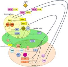


You must be logged in to post a comment.