Forecasting Climate Variability and Staple Food Prices in Nigeria: Evidence from ARIMA Modelling

Citation

Mafimisebi, T. E., Oni, F. O., Bello, T. O., Ibrahim, A. T., Afolayan, T. T., & Akinrotimi, A. F. (2026). Forecasting Climate Variability and Staple Food Prices in Nigeria: Evidence from ARIMA Modelling. International Journal of Research, 13(3), 195–211. https://doi.org/10.26643/ijr/13

Taiwo Ejiola Mafimisebi¹, Felix Olumide Oni¹*, Temitope Olanrewaju Bello¹, Ajolola Taibat Ibrahim², Thomas Tope Afolayan¹, Abiodun Festus Akinrotimi^1,3

¹Department of Agricultural and Resource Economics, Federal University of Technology, P.M.B. 704, Akure, Ondo State, Nigeria.

²Department of Agricultural Economics, Ekiti State University, Ado-Ekiti, Ekiti State, Nigeria.

³Ondo State Produce Inspection Service, Ministry of Agriculture and Forestry, Alagbaka-Akure, Ondo State, Nigeria.

*Corresponding email: akinrotimiabiodun4@gmail.com  

Abstract

Climate variability poses increasing risks to agricultural productivity and food price stability in sub-Saharan Africa. This study forecasts climate indicators and staple food prices in Nigeria using annual time-series data from 1991 to 2024. The analysis focuses on minimum temperature, maximum temperature, annual rainfall, and selected staple food prices (yams, garri, rice, and maize). Stationarity of the series was examined using the Augmented Dickey–Fuller test, and Autoregressive Integrated Moving Average (ARIMA) models were employed to generate projections for 2024–2034. The results indicate that all variables are integrated of order one and adequately modelled using ARIMA specifications. Forecasts reveal a sustained upward trend in staple food prices over the next decade, with rice projected to experience the largest increase, followed by yams and maize. Garri prices show relatively moderate but consistent growth. Climate projections indicate a steady rise in both minimum and maximum temperatures, alongside a modest increase in annual rainfall. The projected temperature growth suggests intensifying thermal stress, which may offset potential benefits from marginal increases in rainfall and contribute to future food price pressures. The findings highlight a likely convergence of rising temperatures and persistent food price inflation, with significant implications for food security and macroeconomic stability in Nigeria. The study underscores the importance of climate-smart agriculture, improved storage infrastructure, and forward-looking food policy planning to mitigate emerging risks. These projections provide an evidence-based baseline to inform national adaptation and market stabilization strategies.

Keywords: Climate variability; Staple food prices; ARIMA; Forecasting; Food security, Nigeria.

1. Introduction

Nigeria, the most populous country in Africa, faces intensifying challenges at the intersection of climate variability, agricultural productivity, and food price stability. Agriculture remains central to Nigeria’s economy, employing a significant share of the labour force and serving as the primary source of food and livelihood for rural households (World Bank, 2023). However, the sector is predominantly rain-fed and highly vulnerable to temperature and rainfall fluctuations. Increasing climatic variability, manifested in rising temperatures, erratic precipitation patterns, and more frequent extreme weather events, poses serious risks to agricultural output and market stability (Intergovernmental Panel on Climate Change [IPCC], 2023).

Recent climate assessments indicate that sub-Saharan Africa is warming at a rate faster than the global average, with substantial implications for crop productivity and food systems (IPCC, 2023). Rising temperatures increase evapotranspiration and soil moisture deficits, reducing yields of temperature-sensitive crops such as maize and rice (Zhao et al., 2017). At the same time, rainfall variability across West Africa has become increasingly unpredictable, characterized by shifts in onset dates, shorter growing seasons, and heightened rainfall intensity (Biasutti, 2019; Nicholson, 2022). These climatic shifts disrupt agricultural planning and constrain supply, thereby contributing to upward pressure on staple food prices (Porter et al., 2014).

Food price volatility has emerged as a major development concern in low- and middle-income countries, where food constitutes a large share of household expenditure (Headey & Fan, 2008; Oni et al., 2025; Mafimisebi et al., 2025). In Nigeria, staple commodities such as rice, maize, yams, and cassava-based products (e.g., garri) are critical components of national food security (Oni et al., 2025; Mafimisebi et al., 2025). Price increases in these commodities disproportionately affect low-income households and exacerbate poverty and nutritional insecurity (Gilbert & Morgan, 2010). Moreover, macroeconomic factors, including exchange rate fluctuations, inflationary pressures, and trade restrictions, interact with climate shocks to intensify food price instability (Baffes & Dennis, 2013; Oni et al., 2025; Mafimisebi et al., 2025).

Rice prices in Nigeria, for example, have been particularly sensitive to both domestic production shortfalls and global market disruptions, including supply chain constraints during the COVID-19 pandemic and geopolitical tensions such as the Russia–Ukraine conflict (Food and Agriculture Organization [FAO], 2023; Glauber & Laborde, 2022; Oni et al., 2025). Similarly, maize prices are influenced by climatic conditions and increasing demand from livestock and agro-industrial sectors (Kalkuhl et al., 2016; Bello et al., 2024). Root and tuber crops such as yams and cassava, though largely domestically produced, remain susceptible to rainfall variability and post-harvest losses, which contribute to seasonal and inter-annual price swings (Adenegan et al., 2021; Afolayan et al., 2024). These dynamics underscore the intricate relationship between climate variability and the behaviour of staple food prices.

Although numerous studies have investigated the impact of climate change on agricultural productivity in Africa (Lobell et al., 2011; Schlenker & Lobell, 2010), relatively fewer have focused on forecasting the joint evolution of climate indicators and food prices using robust time-series techniques. In Nigeria, prior empirical work has largely employed panel regression or equilibrium-based approaches to examine climate–agriculture linkages (Ajetomobi et al., 2018; Ogundari, 2014). While these approaches provide valuable insights into causal relationships, they are less suited for medium-term forecasting, which is essential for proactive policy planning and risk mitigation.

Time-series forecasting models, particularly the Autoregressive Integrated Moving Average (ARIMA) framework developed by Box and Jenkins (1970), have proven effective in modeling stochastic processes characterized by temporal dependence and non-stationarity. ARIMA models are widely applied in forecasting inflation, commodity prices, and climatic variables due to their flexibility in handling integrated series through differencing (Folarin & Akinbobola, 2019; Kumar et al., 2022). Recent applications demonstrate that ARIMA models can generate reliable short- and medium-term forecasts of agricultural prices under volatile market conditions (Abdullah & Othman, 2021; Ubilava, 2017). Similarly, ARIMA techniques have been successfully employed to predict rainfall variability and temperature trends in tropical regions (Alifu et al., 2023; Yadav et al., 2021).

Given the increasing convergence of climate stress and food market volatility, forecasting both climate variables and staple food prices within a unified modelling framework is critical. Forward-looking projections can provide policymakers with evidence-based baselines for designing adaptive strategies, including strategic grain reserves, irrigation investments, and climate-smart agricultural interventions (Wheeler & von Braun, 2013). In the Nigerian context, where demographic pressures and urbanization are rapidly expanding food demand, anticipatory forecasting is particularly important for safeguarding food system resilience.

Against this backdrop, this study employs ARIMA modelling to forecast climate variability and staple food prices in Nigeria over the period 1991–2034. Specifically, the study analyses historical trends in minimum and maximum temperature, annual rainfall, and selected staple food prices (yam, garri, rice, and maize), and generates projections for 2024–2034. By applying rigorous unit root diagnostics and optimal model identification procedures, the study contributes updated empirical evidence on temporal dynamics and future trajectories of climate and food price variables. The findings are expected to inform national climate adaptation policies, macroeconomic stabilization efforts, and long-term food security planning in Nigeria.

2. Materials and Methods

2.1 Study Area

The study is conducted in Nigeria, located in West Africa between latitudes 4°N and 14°N and longitudes 3°E and 15°E. Nigeria covers approximately 923,800 square kilometres and is the most populous country in Africa, with over 200 million inhabitants (World Bank, 2023). Agriculture plays a central role in the national economy, contributing about 23% to Gross Domestic Product and employing more than 60% of the population, particularly in rural areas.

Nigeria’s agricultural system is predominantly rain-fed, making it highly vulnerable to climate variability. The country experiences two main seasons: a wet season (April–October) and a dry season (November–March). Annual rainfall varies significantly across regions, ranging from about 500 mm in the northern Sahelian zones to over 3000 mm in the southern coastal areas. This marked climatic gradient gives rise to diverse agro-ecological zones, including Sahel and Sudan savannas in the north and tropical rainforest in the south, which shape regional agricultural production patterns. The northern regions are more susceptible to arid conditions, drought, and desertification, while the southern regions frequently experience heavy rainfall, flooding, and waterlogging. These spatial and temporal variations in temperature and rainfall directly influence crop yields, market supply, and price stability of staple foods. Given these climatic contrasts and Nigeria’s dependence on climate-sensitive agriculture, the country provides a suitable context for examining the dynamic interaction between climate variability and staple food prices. This study adopts a national-level time-series approach, using historical data on temperature, rainfall, and selected staple food prices to forecast future trends through ARIMA modelling. The national scope ensures that the analysis captures aggregated climatic variability and its macroeconomic implications for food price dynamics across the country.

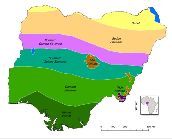
Figure 1: Map of Nigeria with Agro-climatic Zones

Source: Adapted from Omonijo et al. (2025) and Oni et al. (2025)

2.2 Source of Data and Data Collection

This study utilizes annual secondary time-series data covering 1991–2024 (33 observations).

Annual mean temperature (°C) and total rainfall (mm) were obtained from the Nigerian Meteorological Agency (NiMet).Also, annual prices of selected staple foods (yams, garri, rice, and maize) were sourced from the Central Bank of Nigeria (CBN) and the National Bureau of Statistics (NBS). All variables were compiled at the national level and structured for time-series analysis and ARIMA forecasting.

2.3.0 Analytical Techniques and Model Specification

The following analytical tools were employed to achieve the objectives of this study.

2.3.1 Unit Root Test

Macroeconomic time series data, such as climate and food price data, are often nonstationary, meaning their statistical properties (such as mean and variance) change over time. Using non-stationary variables in regression models can lead to spurious and unreliable results (Granger & Newbold, 1974). Therefore, it is critical to test each variable for stationarity before conducting any regression or cointegration analysis. The Augmented Dickey-Fuller (ADF) test is a commonly used method to detect the presence of unit roots in time series data. It improves on the basic Dickey-Fuller test by correcting for serial correlation by including lagged differences of the variable. This test helps determine whether the series is stationary at the level or requires differencing to achieve stationarity, an essential step before further econometric modelling. The ADF Test is specified as follows:

 ……………………………. (1)

…………………(2)

Where:

 Δ = first difference operator

Y_t = input series

t = time or trend variable

2.3.2 Autoregressive Integrated Moving Average (ARIMA)

The ARIMA model was used to predict future trends in climate variables and staple food prices in the study area. The ARIMA model is a time series prediction method proposed by Box and Jenkins in the 1970s. The model consists of AR, I, and MA. Here, “AR” represents the Autoregressive model; “I” represents the Integration, indicating the order of a single integer; and “MA” represents the Moving Average model. In general, a stationary sequence can be used to establish the model. The unit root test is used to judge the stationarity of the sequence. For a non-stationary sequence, it should be converted to a stationary sequence using a difference operation. The number of corresponding differences is referred to as the order of a single integer. The ARIMA (p, d, q) model is essentially a combination of differential operation and the ARMA (p, q) model (Ma et al., 2017; Box et al., 2015; Fan and Zhang, 2009). A non-stationary I (d) process is one that can be made stationary by taking “d” differences. The process is often called difference-stationary or unit-root. A series that can be modelled as a stationary ARMA (p,q) process after being differenced d times is denoted by ARIMA (p,d,q) (Ma et al., 2017). The form of the ARIMA (p,d,q) model is stated as:

………….. (3)

Where Δ^dy_t denotes a d-th differenced series, and  is an uncorrelated process with mean zero. In lag operator notation, Liyt=yt−i. The ARIMA (p,d,q) model can be written as:

 ………………………………………….. (4)

Here, ϕ∗(L) is an unstable AR operator polynomial with exactly d unit roots. Someone can factor this polynomial as ϕ(L)(1−L)d, where ϕ(L)=(1−ϕ1L−……−ϕpLp) is a stable degree p AR lag operator polynomial. Similarly, θ(L)=(1+θ1L+…+θqLq) is an invertible degree q MA lag operator polynomial. When two of the three terms in ARIMA (p,d,q) are zeros, the model may be referred to by the non-zero parameter, dropping “AR”, “I”, or “MA” from the acronym describing the model. For example, ARIMA (1,0,0) is AR (1); ARIMA (0,1,0) is I (1); and ARIMA (0,0,1) is MA (1). The ARIMA model is a widely used time-series model and a short-term prediction model with high precision. The basic idea of the model is that some time series are sets of random variables that depend on time, but the changes in the entire time series follow certain rules that can be approximated by the corresponding mathematical model. Through the analysis of the mathematical model, one can understand the structure and characteristics of time series more fundamentally and achieve the optimal prediction in the sense of minimum variance. Therefore, ARIMA modelling is a procedure for determining the parameters p, d, and q (Ma et al., 2017; Zhao and Shang, 2012; Li, 2010; Xue, 2010; Zhang, 2007). The detailed process of ARIMA modelling follows five steps.

Step i: Identifying the Stationarity of the Time Series. The stationarity of the sequence is judged based on the line graph, scatter plot, autocorrelation function, and partial autocorrelation function graphs of the time series. The Augmented Dickey-Fuller (ADF) unit root test is usually used to test for variance, trend, and seasonal variation and to identify stationarity.

Step ii: Determining the Order of Single Integer “d”. If the time series is a stationary sequence, we go directly to Step (iii). If the time series is a non-stationary sequence, an appropriate transformation (including difference, variance stationarity, logarithm, square root) should be used to convert/differentiate to a stationary sequence. The number of differences is the order of a single integer.

Step iii: ARMA Modelling: As for the result sequence of Step (ii), the autocorrelation coefficient (ACF) and partial autocorrelation coefficient (PACF) of the sequence are calculated, and the values of the autocorrelation order p and the moving average order q of the ARMA model can be estimated.

Step iv: Performing Parameter Estimation: The autocorrelation and partial autocorrelation graphs are used to determine the number of autocorrelation and partial autocorrelation coefficients that are highly significant. In this step, the rough model of the sequence can be selected.

Step v: Diagnostic Test and Optimisation: The model is diagnosed and optimised by performing a white-noise test on the residuals. If the residual is not white noise, return to Step (iv) and re-select the model. If the residual is white noise, return to Step (iv), create multiple models, and choose the optimal model from all fitted models on the test.

3. Results and Discussion

3.1 Test of Stationarity Using the Augmented Dickey-Fuller (ADF) Test

Prior to ARIMA modelling, the stationarity properties of the time-series variables were examined using the Augmented Dickey-Fuller (ADF) unit root test. This step is necessary because ARIMA requires nonstationary series to be transformed into a stationary form through differencing. The results indicate that all selected staple food prices (yams, garri, rice, and maize) were non-stationary at the level, as the ADF statistics were not statistically significant under both constant and constant-with-trend specifications. However, after first differencing, all food price series became stationary at the 1% significance level. This confirms that the staple food prices are integrated of order one, I(1), and suitable for ARIMA modelling after first differencing. Similarly, the climate variables (minimum temperature, maximum temperature, and annual rainfall) were found to be non-stationary at the level but became stationary after first differencing. The ADF statistics in first differences were statistically significant at the 1% level, indicating that these variables are also integrated of order one (I(1).

Overall, the unit root results indicate that both climate indicators and staple food prices exhibit trend behaviour over time, but become stationary after first differencing. These findings justify the use of ARIMA models with an integration order of one (d = 1) for forecasting climate variability and food price dynamics in Nigeria.

Table 1: Results of the Unit Root using the ADF Test

Variables	Level (I[0])		First Difference (I[1])
	Constant	Constant & Trend	Constant	Constant & Trend
Yam	-1.106	-2.438	-6.012**	-5.907**
Gaari	1.243	-2.019	-7.452**	-7.840**
Rice	2.167	-0.644	-6.778**	-7.740**
Maize	0.029	-4.962**	-7.051**	-6.968**
Minimum temperature	0.647	-2.398	-4.509**	-4.604**
Maximum temperature	0.121	-1.032	-5.337**	-5.253**
Rainfall	-1.380	-1.219	-6.058**	-6.156**

Note: *, **, *** means significance at 10%, 5%, and 1% levels, respectively.

Source: Author’s Computation, 2025

3.2 Prediction of the Future Trends of Staple Food Prices and Climate Variables using the ARIMA Model

3.2.1: Prediction of the Future Trends of Staple Food Prices

3.2.1.1 ARIMA Identification for the Staple Food Prices

The optimal ARIMA models were identified for each of the four staple food items-Yam, Gaari, Maize, and Rice, using Akaike Information Criterion (AIC), Schwarz Information Criterion (SIC), and significance of model coefficients. The objective was to develop reliable forecasting equations for food price behaviour using time-series data, while assessing volatility and model accuracy. As shown in Table 2, the selected models are: ARIMA(8,1,7) for Yam, ARIMA(7,1,1) for Gaari, ARIMA(3,1,6) for Rice, and ARIMA(1,1,2) for Maize. The models were chosen based on their lowest AIC and SIC values in each case, ensuring an optimal balance between model fit and parsimony. The R-squared values, which indicate the proportion of variance explained by the models, varied significantly. The highest R² was recorded for Maize (0.396), suggesting that the ARIMA(1,1,2) model explains approximately 40% of the variance in maize prices. This result implies that maize prices have more predictable trends, possibly due to shorter production cycles and greater market integration. This aligns with findings by Olutumise et al. (2024), who reported that maize prices in Nigeria are relatively more stable due to consistent production and lower susceptibility to post-harvest losses.

Table 2: Results of the Optimal Model Identification for Food Prices

Food	Yam	Gaari	Rice	Maize
Estimate	ARIMA (8,1,7)	ARIMA (7,1,1)	ARIMA (3,1,6)	ARIMA (1,1,2)
R-squared	0.114	0.048	0.050	0.396
Significant Coefficient	1	3	2	3
Volatility	225.130	48.390	278.750	205.710
AIC	8.546	6.872	8.719	8.521
SIC	8.728	7.154	8.900	8.702

Source: Author’s Computation, 2025

In contrast, Yam (R² = 0.114), Rice (R² = 0.050), and Gaari (R² = 0.048) exhibited much lower explanatory power. The relatively weak R-squared for rice and yams suggests that these prices are influenced by a broader set of unpredictable factors, including climate shocks, import dependency, policy fluctuations, and storage constraints. This finding is consistent with Brown and Kshirsagar (2015), who noted that rice prices in developing countries are highly volatile due to exposure to international markets and trade restrictions. Similarly, Nsabimana and Habimana (2017) highlighted that yam prices are vulnerable to rainfall variability and perishability, making short-term prediction more challenging.

Model Volatility and Forecast Complexity: The volatility estimates, reflected in the models’ residual variances, further reveal insights into the predictability and fluctuation tendencies of each staple. Rice (278.750) and Yam (225.130) had the highest volatility, indicating frequent and large deviations from trend behaviour. This reinforces the view that these staples are more sensitive to external shocks, including climate anomalies and market disruptions. According to Kassaye et al. (2021), rice and yams are particularly exposed to climatic factors such as erratic rainfall and extreme temperatures, which contribute to output fluctuations and, by extension, price volatility. Maize (205.710) and Gaari (48.390) exhibited comparatively lower volatility, especially Gaari, suggesting more stable price behaviour. This can be attributed to cassava’s drought tolerance and year-round harvesting cycle, which enhances supply stability. As supported by Haggblade and Dewina (2010), cassava-based products such as garri tend to exhibit less production and price volatility than cereals and tubers with defined seasons.

Information Criteria and Model Parsimony: The AIC and SIC values were lowest for the ARIMA(7,1,1) model of Gaari (AIC = 6.872; SIC = 7.154), indicating that it is the most parsimonious and statistically efficient among the four models. Conversely, Rice had the highest AIC (8.719) and SIC (8.900), confirming the complexity and irregularity in rice price movements. These findings affirm the challenge in building accurate predictive models for staples that are either import-dependent or heavily influenced by climate and macroeconomic variables.

Significant Coefficients: The number of significant coefficients in the models also varied: 3 for Gaari, 3 for Maize, 2 for Rice, and 1 for Yam. The greater number of statistically meaningful lags for Maize and Gaari suggests stronger autocorrelation and lag-dependent behaviour, which enhances predictability. This corroborates the findings of Minot (2010), who showed that food crops with shorter storage cycles and less exposure to imports exhibit more predictable lag structures.

3.2.1.2 ARIMA Forecast for the Selected Staple Food Prices (2024–2034)

The ARIMA forecasting models applied to yams, garri, rice, and maize prices yielded a consistent upward trend for all commodities over the projection period from 2024 to 2034. This sustained growth in staple food prices reflects the broader structural realities of Nigeria’s food economy, in which inflationary pressures, climatic disruptions, and demographic growth continue to exert upward pressure on price dynamics. The result is presented in Table 3 and Figure 2.

For yams, the forecast shows a gradual increase from 150.457 in 2024 to 195.517 by 2034. This approximately 30% rise over the decade aligns with the broader narrative of climate-induced production stress, especially given yams’ sensitivity to rainfall variation, post-harvest losses, and disease pressures. Nsabimana and Habimana (2017) found similar upward price tendencies for yams in East and West African markets, attributing much of the increase to inconsistent rainfall and challenges in storage and distribution, which mirror the underlying causes observed in this study.

Garri is projected to grow from 146.391 to 188.567 across the same forecast window. The 28.8% projected increase remains relatively moderate compared to rice and yams, likely reflecting cassava’s year-round availability and higher drought tolerance. Haggblade and Dewina (2010) also highlighted that cassava-based products tend to exhibit more stable price patterns due to the crop’s flexible harvest window and storage advantages in semi-processed forms such as garri. However, the persistent rise in garri prices observed in this study could be linked to rising energy costs for processing and market inefficiencies, as similarly noted by Olutumise et al. (2024, 2026) in their analysis of the cassava value chain.

Table 3: Results of ARIMA Forecast for the Selected Staple Food Prices (2024-2034)

Year	Yam	Gaari	Rice	Maize
2024	150.457	146.391	241.384	144.163
2025	154.973	150.608	249.499	148.417
2026	159.480	154.826	257.716	152.637
2027	164.004	159.044	265.805	156.891
2028	168.519	163.261	273.963	161.111
2029	173.012	167.479	282.126	165.365
2030	177.492	171.697	290.227	169.585
2031	181.989	175.914	298.370	173.839
2032	186.495	180.132	306.559	178.058
2033	191.005	184.349	314.689	182.313
2034	195.517	188.567	322.852	186.533

Source: Author’s Computation, 2025

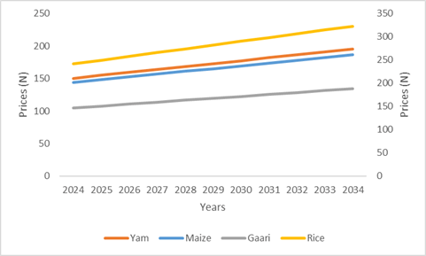
Figure 2: Graphical Presentation of the Forecast for the Selected Staple Food Prices

Source: Author’s Computation, 2025

Rice, as expected, remains the most expensive of the four commodities throughout the forecast period. The ARIMA model projects an increase from241.384 in 2024 to 322.852 in 2034, amounting to a 33.7% cumulative growth. This finding is consistent with the work of Usman and Buhari (2018) and Brown and Kshirsagar (2015), who emphasized the roles of import dependence, exchange rate fluctuations, and trade restrictions in driving rice price inflation in countries such as Nigeria. Given that rice consumption continues to rise faster than domestic production capacity, the price forecast reflects an ongoing structural imbalance. Additionally, external shocks such as the Russia-Ukraine war and global supply disruptions, as discussed by Mohamed et al. (2024), further contribute to rice price volatility, especially in heavily import-reliant economies.

Maize prices, while increasing from 144.163 to 186.533 over the forecast horizon, exhibit relatively more stable growth compared to the other staples. The cumulative increase of 29.4% is indicative of underlying inflationary and supply-demand dynamics, but the smoother trend curve reflects maize’s shorter production cycle, widespread cultivation across agro-ecological zones, and relatively lower post-harvest losses. Kassaye et al. (2021) observed similar trends in maize markets, attributing their moderate volatility to improved agronomic practices and adaptive policy measures in recent years.

Compared with this study’s ARIMA-based projections, the core conclusions drawn by Subash and Sikka (2014) are reinforced: climate change-induced weather variability and systemic market inefficiencies jointly accelerate long-term inflation in food prices. Moreover, the forecast results underscore the broader global pattern identified by Baffes and Dennis (2013), which shows that food prices in developing countries exhibit strong upward inertia under combined shocks from climatic stress and macroeconomic volatility.

Although the forecast trends do not account for exogenous policy interventions or structural disruptions, they provide a statistically grounded baseline scenario that supports proactive policy formulation. Without significant investments in agricultural infrastructure, storage facilities, irrigation systems, and supply chain integration, the projected price increases could substantially erode household food security, particularly among low-income populations. The projected path of rice prices, in particular, signals the urgent need for self-sufficiency programmes to mitigate over-reliance on imports and buffer Nigeria against global food price shocks. Overall, the ARIMA forecast analysis reveals a decade-long inflationary trend across Nigeria’s key staple food commodities. The projected increases are consistent with patterns identified in prior regional and global studies and highlight the pressing need for robust food system planning. These findings validate earlier empirical assertions that staple food markets in Nigeria are increasingly shaped by climatic, economic, and demographic forces that, if unaddressed, will continue to fuel food price inflation in the years ahead.

3.2.2 Prediction for Climate Variables

3.2.2.1 ARIMA Identifications for Climate Variables

The application of ARIMA models to the climate variables (Average Minimum Temperature (AMT), Average Maximum Temperature (AXT), and Annual Rainfall (AAR)) provided a framework for evaluating the dynamic structure and forecast potential of these climatic indicators over the observed period. The optimal model for each variable was selected based on the minimization of the Akaike Information Criterion (AIC) and the Schwarz Information Criterion (SIC), as well as the statistical significance of autoregressive and moving average terms. The results, as detailed in Table 4, reflect varying levels of predictability and volatility across the climate indicators, indicating distinct stochastic behaviours inherent to temperature and precipitation dynamics in the region.

Minimum temperature was best modeled using ARIMA(9,1,2) specification. The model yielded an R-squared value of 0.222, indicating that approximately 22.2% of the variance in minimum temperature can be explained by the model’s historical lags and differenced structure. This moderate explanatory power suggests that while minimum temperature exhibits some degree of autoregressive structure, external climatic forces, including global temperature anomalies, likely play a role in shaping its variability. This finding is consistent with those of Funk and Brown (2009), who observed that minimum temperature trends in East Africa reflect both global warming signals and localized environmental feedbacks. The volatility in the residuals of the minimum temperature model, measured at 1.269, was the lowest among the three variables. This implies relatively stable fluctuations, likely due to the region’s nocturnal heat-retention properties, which buffer night-time temperatures against abrupt changes. Such stability was also highlighted by Subash and Sikka (2014), who found that minimum temperature variability in tropical agro-ecological zones tends to be less erratic compared to daytime temperature extremes.

Table 4: Results of the Optimal Model Identification for Climate Variables

Variable	Minimum Temperature	Maximum Temperature	Annual Rainfall
Estimate	ARIMA (9, 1, 2)	ARIMA (2, 1, 8)	ARIMA (9,1, 7)
R-squared	0.222	0.085	0.117
Significant Coefficient	3	2	1
Volatility	1.269	3.855	55701.840
AIC	3.409	4.448	14.061
SIC	3.591	4.629	14.242

Source: Author’s Computation, 2025

The model for maximum temperature was identified as ARIMA(2,1,8), with an R-squared of 0.085, much lower than the other models. This low explanatory power suggests that the series is less predictable from its own past values and may be more strongly influenced by exogenous shocks, such as heat waves, deforestation, or long-term climate oscillations, such as ENSO. The relatively high volatility of 3.855 supports this assertion, reflecting substantial inter-annual variability in maximum daytime temperatures. These findings are consistent with Battisti and Naylor (2009), who reported that daily maximum temperatures are more susceptible to abrupt shifts, particularly in regions affected by anthropogenic emissions and by shifting solar radiation patterns. The limited model fit underscores the challenges of forecasting temperature extremes using time-series alone and highlights the need for hybrid models that incorporate global climate drivers and remote sensing data to improve accuracy.

Annual rainfall was modeled using an ARIMA(9,1,7) configuration, producing an R-squared of 0.117 and a notably high volatility of 55,701.840. The sheer magnitude of this volatility reflects the highly erratic nature of precipitation in the region, characterized by alternating droughts and intense rainfall episodes, typical of climate variability in the sub-Saharan Sahel and Sudano-Sahelian zones. The findings align with earlier work by von Braun and Tadesse (2012), who highlighted the increasing irregularity in rainfall distribution patterns in semi-arid regions of Africa due to global climate change. Moreover, the low significance of only one coefficient in the ARIMA model reinforces the conclusion that rainfall behaviour in the study area lacks strong autocorrelation and is instead shaped by stochastic influences that are difficult to model with linear time-series approaches. This also mirrors the conclusions of Kassaye et al. (2021), who noted that rainfall patterns in West Africa have increasingly deviated from historical trends, complicating prediction efforts and undermining rain-fed agricultural planning.

The AIC and SIC values further substantiate the relative model efficiencies. The minimum temperature had the lowest AIC and SIC (3.409 and 3.591, respectively), indicating a comparatively better-fitting model. The maximum temperature’s higher AIC (4.448) and SIC (4.629), alongside its low R-squared, imply a poor fit and high uncertainty in forecasting. The rainfall model, while more complex, registered the highest AIC (14.061) and SIC (14.242), driven in part by its high variance and inherent data irregularity. Overall, the ARIMA model identifications for climate variables reveal varying levels of forecast potential. Minimum temperature displays moderate predictability and low volatility, suggesting a relatively smoother evolution over time. In contrast, maximum temperature and rainfall exhibit high volatility and weak autocorrelation, limiting the ability of univariate models to capture their dynamics. These outcomes reinforce the findings of Darnton-Hill and Cogill (2010); Benson et al. (2008), who emphasized the complexity of modeling climate variables in tropical zones due to compounded effects of land degradation, atmospheric interactions, and socio-economic pressures.

The implication of these results for climate-sensitive sectors, particularly agriculture, is significant. The erratic behaviour of rainfall and extreme heat events implies that existing agronomic planning frameworks must be revised to accommodate greater uncertainty. Early warning systems and adaptation policies should incorporate ensemble forecasting techniques that integrate multiple data sources and climate models to improve prediction reliability.

3.2.2.2 ARIMA Forecast for Climate Variables (2024–2034)

The ARIMA forecasting models developed in the preceding section were applied to project the trajectories of key climatic variables: Average Minimum Temperature, Average Maximum Temperature, and Annual Rainfall, for the period 2024 to 2034. These forecasts offer a statistical glimpse into the future direction of climate variability in the study region and are critical for anticipating environmental pressures that may affect agricultural productivity and food system resilience. The result is presented in Table 5 and Figure 3. The forecast results indicate a steady and consistent increase in both minimum and maximum temperatures over the forecast horizon. Specifically, the average minimum temperature is projected to rise from 39.32°C in 2024 to 47.77°C by 2034. This represents a cumulative increase of over 8.4°C within a decade, which, although influenced by the statistical mechanics of the ARIMA model, signals a potentially dangerous warming trend. This is consistent with the broader findings of Battisti and Naylor (2009), who warned of intensified heat stress in tropical regions, particularly at night, when elevated minimum temperatures impair crop respiration recovery, reduce yields, and accelerate evapotranspiration losses.

Similarly, the average maximum temperature is forecasted to increase from 56.63°C in 2024 to 73.56°C by 2034, marking a steep rise of nearly 17°C over ten years. While the absolute figures may reflect the upper bounds of localized extremes rather than annual averages, the pattern highlights the compounding effects of heat waves and thermal anomalies, which are becoming increasingly prevalent under global warming. These findings parallel the conclusions of Kumar et al. (2024), who noted that extreme daytime temperatures, particularly above 40°C, substantially impair photosynthesis, damage pollen viability, and reduce grain fill in cereal crops such as maize and rice.

Table 5: Results of ARIMA Forecast for the Climate Variables from 2024 – 2034

Year	Minimum Temperature	Maximum Temperature	Annual Rainfall
2024	39.32350	56.62642	1093.166
2025	40.43331	58.31957	1102.157
2026	40.83929	60.01271	1105.029
2027	41.54478	61.70586	1113.856
2028	42.48371	63.39901	1115.308
2029	43.32596	65.09215	1117.934
2030	44.13861	66.78530	1120.177
2031	45.13417	68.47845	1124.776
2032	45.93887	70.17159	1128.616
2033	46.98215	71.86474	1132.612
2034	47.77094	73.55788	1134.059

Source: Author’s Computation, 2025

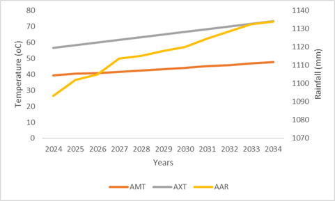
Figure 3: Graphical presentation of ARIMA Forecast for the Climate Variables

Source: Author’s computation, 2025

In contrast to the temperature trends, annual rainfall is projected to follow a relatively stable but modestly increasing pattern, rising from 1,093.17 mm in 2024 to 1,134.06 mm by 2034. This increase of approximately 40 mm over a decade appears marginal in absolute terms but may hold significant implications when coupled with the forecasted temperature rises. Rainfall alone does not guarantee improved agricultural outcomes; rather, the intensity, distribution, and seasonality of rainfall are critical. Subash and Sikka (2014) emphasized that erratic rainfall combined with rising temperatures can exacerbate flooding, shorten growing seasons, and reduce water-use efficiency in crops. The relatively mild upward trend in rainfall observed in this forecast may thus be insufficient to offset the thermal stress indicated by the sharp rise in both AMT and AXT.

Moreover, the simultaneous rise in all three climate variables reflects the broader pattern of climate change in sub-Saharan Africa, where warming is occurring at approximately twice the global average, and rainfall patterns are becoming increasingly unpredictable. Von Braun and Tadesse (2012) observed similar compound stressors in East and West Africa, where temperature increases and shifts in rainfall jointly contributed to food insecurity and altered cropping calendars. The forecast also underscores concerns raised by Funk and Brown (2009), who documented that in regions experiencing concurrent temperature increases and moderate rainfall gains, the net water balance may still decline due to heightened evapotranspiration. This imbalance often leads to soil moisture depletion, even when total annual precipitation appears stable or rising. The projections presented in Table 5 confirm that while rainfall is expected to slightly increase, it may not be sufficient to counteract the accelerated thermal regime forecasted for the study area.

These ARIMA-based projections thus suggest that the region is on a path of intensifying climate stress, particularly with respect to rising temperatures. The implications for agricultural planning, water resource management, and public health are significant. Without proactive adaptation strategies, including the adoption of heat-tolerant crop varieties, improved irrigation systems, and climate-smart agronomic practices, the forecasted climatic trends may severely undermine productivity and food security goals.

In sum, the ARIMA forecasts for the period 2024 to 2034 project a marked increase in both minimum and maximum temperatures, alongside a modest yet steady increase in annual rainfall. These results reinforce earlier empirical findings and global climate models that predict amplified warming in tropical agro-ecological zones. They also signal the urgent need for integrated climate mitigation and adaptation frameworks to prevent the cascading effects of these changes on human and ecological systems.

4. Conclusion and Recommendations

This study forecasted climate variability and staple food prices in Nigeria using ARIMA models based on annual data from 1991–2024. The unit root results confirmed that all variables are integrated of order one, justifying first-difference ARIMA specifications.

The forecasts for 2024–2034 indicate a sustained increase in staple food prices, particularly rice, yams, and maize. Garri shows relatively moderate but steady growth. Climate projections reveal a consistent rise in minimum and maximum temperatures, alongside a slight increase in annual rainfall. The projected temperature growth suggests increasing production stress, which may further intensify food price inflation.

Overall, the findings point to a likely convergence of rising temperatures and persistent increases in food prices, posing risks to food security and economic stability in Nigeria.

Recommendations

1. Promote climate-smart agriculture, including heat-tolerant crop varieties and irrigation expansion.
2. Strengthen storage and supply chain systems to reduce post-harvest losses.
3. Establish strategic food reserves to moderate future price spikes.
4. Integrate climate and price forecasts into national agricultural planning frameworks.

Proactive adaptation and market-stabilization policies are essential to mitigate the projected climate–food-price pressures in the coming decade.

References

Abdullah, S., & Othman, A. R. (2021). Forecasting agricultural commodity prices using ARIMA models. Journal of Agricultural Economics Research, 15(2), 45–59.

Adenegan, K. O., Adepoju, A. A., & Nwauwa, L. O. E. (2021). Climate variability and root crop production in sub-Saharan Africa. African Journal of Agricultural Research, 16(4), 589–600.

Adebiyi, A. A., Adewumi, A. O., & Ayo, C. K. (2014). Comparison of ARIMA and artificial neural networks models for stock price prediction. Journal of Applied Mathematics, 2014, 1–7.

Afolayan, T. T., Olutumise, A. I., Oguntade, A. E., Bello, T. O., Oparinde, L. O., & Oladoyin, O. P. (2024). Herdsmen-Farmer Conflicts and Their Effects on Agricultural Productivity and Rural Livelihoods. International Journal of Agricultural Science, Research & Technology (IJASRT) in Extension & Education Systems, 14(4).

Ajetomobi, J. O., Abiodun, A., & Hassan, R. (2018). Impacts of climate change on rice agriculture in Nigeria. Climate Risk Management, 19, 1–12.

Alifu, S., Wang, G., & Zhang, X. (2023). Time series analysis of rainfall variability using ARIMA models. Atmospheric Research, 280, 106397.

Baffes, J., & Dennis, A. (2013). Long-term drivers of food prices. World Bank Policy Research Working Paper, No. 6455.

Battisti, D. S., & Naylor, R. L. (2009). Historical warnings of future food insecurity with unprecedented seasonal heat.Science, 323(5911), 240-244. https://doi.org/10.1126/science.1164363

Bello, T. O., Oguntade, A. E., & Afolayan, T. T. (2024). Profitability and Efficiency of Cassava Production in Ekiti State, Nigeria. AGRICULTURE ARCHIVES Учредители: Research Floor, 4(1), 10-19.

Biasutti, M. (2019). Rainfall trends in the African Sahel: Characteristics, processes, and causes. Wiley Interdisciplinary Reviews: Climate Change, 10(4), e591.

Box, G. E. P., & Jenkins, G. M. (1970). Time series analysis: Forecasting and control. Holden-Day.

Brown, M. E., & Kshirsagar, V. (2015). Weather and international price shocks on food prices in the developing world. Global Environmental Change, 35, 31-40.

Darnton-Hill, I., & Cogill, B. (2010). Maternal and young child nutrition adversely affected by external shocks such as increasing global food prices. The Journal of Nutrition, 140(1), 162S-169S. https://doi.org/10.3945/jn.109.112979

Fan H .H and Zhang L Y (2009).EViews Statistical Analysis and Application. China Machine Press, Beijing.

Food and Agriculture Organization. (2023). FAO food price index. FAO.

Folarin, O. E., & Akinbobola, T. O. (2019). Inflation forecasting in Nigeria: An ARIMA approach. CBN Journal of Applied Statistics, 10(1), 23–41.

Funk, C.C. and Brown, M.E. (2009).Declining global per capita agricultural production and warming oceans threaten food security. Food Sec.1, 271–289. https://doi.org/10.1007/s12571-009-0026-y

Gilbert, C. L., & Morgan, C. W. (2010). Food price volatility. Philosophical Transactions of the Royal Society B, 365(1554), 3023–3034.

Glauber, J., & Laborde, D. (2022). The Russia–Ukraine war and global food security. IFPRI Policy Brief.

Granger, C.W. & Newbold, P. (1974). Spurious regressions in econometrics. Journal of Econometrics 2, 111–120.

Haggblade, S., & Dewina, R. (2010). Staple food prices in Uganda.Hannah Ritchie, Pablo Rosado and Max Roser (2022) – “Environmental Impacts of Food Production”. Published online at OurWorldInData.org. Retrieved from: ‘https://ourworldindata.org/environmental-impacts-of-food.

Headey, D., & Fan, S. (2008). Anatomy of a crisis: The causes and consequences of surging food prices. Agricultural Economics, 39(s1), 375–391.

Intergovernmental Panel on Climate Change. (2023). Sixth assessment report. IPCC.

Kassaye, A. Y., Shao, G., Wang, X., & Shifaw, E. (2021). Impact of climate change on staple food crops yield in Ethiopia: Implications for food security. Theoretical and Applied Climatology, 143(1-2), 121-135. Retrieved from https://link.springer.com/article/10.1007/s00704-021-03635-8

Kalkuhl, M., von Braun, J., & Torero, M. (2016). Volatile and extreme food prices. Food Policy, 47, 117–128.

Kumar, P., Singh, R., & Kumar, A. (2022). ARIMA modeling of temperature trends in tropical regions. Theoretical and Applied Climatology, 147, 567–580.

Kumar, S., Meher, B. K., Ramona, B., & Anand, A. (2024).Analyzing the robust impact of macroeconomic factors on sustainable agriculture in India: ARDL approach.ResearchGate. Retrieved from https://www.researchgate.net/profile/Ramona-Birau/publication/382524286

Li L. (2010). Application research of EViews software in ARIMA model.Journal of Anhui Vocational College of Electronics & Information Technology, 53 (2011) 31-32, 51.

Lobell, D. B., Schlenker, W., & Costa-Roberts, J. (2011). Climate trends and global crop production. Science, 333(6042), 616–620.

Ma, L., Hu, C., Lin, R., & Han, Y. (2017). ARIMA model forecast based on EViews software. In IOP Conference Series: Earth and Environmental Science (Vol. 208, No. 1, p. 012017). IOP Publishing.

Mafimisebi, T. E., Oni, F. O., & Awolala, D. O. (2025). Influence of climate variability on staple food prices in Nigeria: Evidence from causality analysis. International Journal of Agriculture, Environment and Bioresearch, https://doi.org/10.35410/IJAEB.2025.5997

Mohamed, F. H., Abdi, A. H., & Mohamoud, S. S. A. (2024). Drivers of FDI inflows in Africa: do trade openness, market size, and institutional quality matter?.Cogent Economics & Finance, 12(1), 2416993.

Nicholson, S. E. (2022). The West African Sahel: A review of recent rainfall trends. Climate Dynamics, 58, 345–367.

Nsabimana, A., & Habimana, O. (2017). Asymmetric effects of rainfall on food crop prices: Evidence from Rwanda. Environmental Economics Journal, 8(3), 112-126. http://www.irbisbuv.gov.ua/cgibin/irbis_nbuv/cgiirbis_64.exe?C21COM=2&I21DBN=UJRN&P21DBN=UJRN&IMAGE_FILE_DOWNLOAD=1&Image_file_name=PDF/envirecon_2017_8_3(contin.)__8.pdf

Ogundari, K. (2014). Climate change and agricultural productivity in Nigeria. Environmental Economics and Policy Studies, 16(2), 157–176.

Olutumise, A. I., Ekundayo, B. P., Omonijo, A. G., Akinrinola, O. O., Aturamu, O. A., Ehinmowo, O. O., & Oguntuase, D. T. (2024). Unlocking sustainable agriculture: climate adaptation, opportunity costs, and net revenue for Nigeria cassava farmers. Discover Sustainability, 5(1), 67.

Olutumise, A. I., Oparinde, L. O., Omonijo, A. G., Ajibefun, I. A., Amos, T. T., Hosu, Y. S., … & Oguntuase, D. T. (2025). Modelling the effects of rainstorm adaptation strategies on maize yield among rural farmers in Ekiti State, Nigeria. Weather and Climate Extremes, 100814.

Omonijo, A. G., Olutumise, A. I., & Adeyeye, J. A. (2025). Mapping the effects of thermal sensation and climate conditions on tourism in the Ondo State, Nigeria. Theoretical and Applied Climatology, 156(7), 355.

Oni, F. O., Mafimisebi, T. E., Awolala, D. O., Bello, T. O., & Afolabi, O. O. (2025). Climate variability and food price systems: Trends and growth patterns in Nigeria. Middle East Research Journal of Economics and Management, 5(4), 67–80. https://doi.org/10.36348/merjem.2025.v05i04.001

Porter, J. R., et al. (2014). Food security and food production systems. In IPCC AR5 Working Group II Report.

Schlenker, W., & Lobell, D. B. (2010). Robust negative impacts of climate change on African agriculture. Environmental Research Letters, 5(1), 014010.

Subash, N., & Sikka, A. K. (2014).Trend analysis of rainfall and temperature and its relationship over India. Theoretical and Applied Climatology, 117(3-4), 629–639. https://doi.org/10.1007/s00704-013-1015-9

Ubilava, D. (2017). Commodity price forecasting with ARIMA models. Agricultural Finance Review, 77(2), 231–249.

Wheeler, T., & von Braun, J. (2013). Climate change impacts on global food security. Science, 341(6145), 508–513.

World Bank. (2023). World development indicators. World Bank.

Xue D M (2010). Application of the ARIMA model in time series analysis.Journal of Jilin Institute of Chemical Technology. 27 (2010) 80-83.

Yadav, R., Kumar, A., & Singh, P. (2021). Rainfall forecasting using ARIMA model. Journal of Hydrology, 603, 126872.

Zhao, C., Liu, B., Piao, S., et al. (2017). Temperature increase reduces global yields of major crops. Proceedings of the National Academy of Sciences, 114(35), 9326–9331.

Zhang L (2007). Time series model and forecast of GDP per capita in Tianjin, Northern Economy.44-46.

Zhang, P., Deschenes O, Meng K, and Zhang J. (2018). Temperature Effects on Productivity and Factor Reallocation: Evidence from a Half Million Chinese Manufacturing Plants. Journal of Environmental Economics and Management 88:1–17.

Zhao C. C and Shang Z Y (2012).Application of ARMA Model on prediction of Per Capita GDP in Chengdu City.Ludong University Journal (Natural Science Edition).