Office wall art should look orderly and stay secure. This guide covers safe mounting heights, clean spacing, and hardware choices for an office canvas print setup that works in busy workspaces.
Plan the Layout First
Measure the wall and nearby furniture
Measure the wall, then note what sits under it: desks, credenzas, benches, or a reception counter. Check door swings and walk paths so artwork corners are not in the way.
Before you plan the final placement, identify the wall surface (drywall, brick, concrete, or glass partition) and confirm what your building allows. Many offices also have hidden cable runs and sensors. A quick scan with a stud finder and a look at building drawings can prevent drilling into something you should not touch.
Choose the right size for the wall
One larger piece often reads cleanly in a focused work zone. Longer walls can handle a set of two or three pieces when the gaps are consistent. A helpful sizing check is to keep the full artwork width around two-thirds to three-quarters of the furniture width below it.
For meeting rooms, hallways, and workstations, explore Office Canvas Prints and pick a size that matches the wall width and viewing distance. If people mainly view the wall while seated, keep the center slightly lower than a standing-height corridor.
Mock up before you drill
Tape paper templates to the wall and step back to where people will view the art. Adjust until the placement feels centered and straight next to furniture and lighting. For sets, label templates so you do not mix up the order when you start drilling.
Standard Mounting Heights That Work in Offices
Use the eye-level center rule
A solid starting point is to place the center of the artwork around 57–60 inches (145–152 cm) from the floor. Keep a similar center line across a room so walls feel organized.
Hang art above desks and credenzas
When artwork sits above furniture, keep the bottom edge about 6–10 inches (15–25 cm) above the top surface. If the furniture is tall, start closer to 6 inches so the art does not drift too high.
Reception areas and corridors
In reception areas, use the same center-height approach rather than pushing art upward for tall ceilings. In hallways, leave enough side clearance so bags and shoulders do not brush the edges.
Spacing Rules for Single Pieces and Groupings
Single piece spacing
Give a single office art print room from trim, corners, and shelving. If the wall has switches or thermostats, keep the art far enough away that the wall does not feel crowded.
Two- and three-piece sets
Keep gaps consistent. A 2–4 inch (5–10 cm) gap between canvases works well on office walls. Measure edge to edge and check the gap in more than one spot before tightening hardware.
To center a set, calculate the full width of the group (all pieces plus the gaps), then mark the midpoint on the wall. Work outward from that center mark. If you have a laser level, use it to keep the top edges aligned across the full group.
Gallery-style layouts
Pick one alignment system—top edges, bottom edges, or a shared center line—and follow it across the whole group. If you are mixing sizes, build from the center outward so the group stays centered.
Hardware Choices for Safe Installation
Studs, anchors, and weight limits
Use studs when you can, especially for heavier pieces. If studs are not available where you need them, choose heavy-duty anchors made for your wall type and follow the rated limits on the packaging. When in doubt, select hardware rated well above the artwork weight to allow a safety buffer.
Hanging methods that reduce shifting
Two-point hanging helps keep frames from tilting. For larger pieces, French cleats can hold the art flatter to the wall and reduce movement in busy areas. Small bumpers on the lower corners can also help keep frames steady.
Alternatives for offices that change layouts often
If your office refreshes walls regularly, a rail-and-cable system can reduce wall damage because you adjust hooks rather than drill new holes. This approach is common in hallways and reception zones where artwork is updated seasonally or for events.
Match art to client-facing spaces
For conference rooms and reception walls, themes like leadership, teamwork, and growth fit many workplaces. If you want pieces built around these ideas, browse Business Concept Canvas Prints and choose sizes that suit your room scale.
Lighting and Glare Checks
Check the wall with lights on and at different times of day. Windows and strong overhead fixtures can create glare. If needed, shift the art a little or adjust nearby lighting angles.
Tools and Materials You’ll Want Ready
Tape measure, pencil, and painter’s tape
Level (or a leveling app)
Stud finder
Drill/driver, screws, and wall anchors
Step stool or ladder approved for your workplace
Step-by-Step Office Art Installation Workflow
Mark the center height. Lightly mark where the artwork center should sit.
Measure the hanging offset. Measure from the top of the frame to the hook point on the back.
Set hardware. Use studs when possible; otherwise install anchors rated for the weight.
Hang and level. Hang the piece, level it, then tighten hardware and recheck.
Verify clearance. Open nearby doors, roll a chair back, and confirm nothing catches the frame.
For grouped pieces, hang the center piece first (or the center line for a grid), then work outward. Step back to the normal viewing distance and confirm the gaps read evenly from that angle.
Quick Rules for Clean Placement
Keep the artwork center near 57–60 inches (145–152 cm) from the floor.
Above furniture, keep the bottom edge about 6–10 inches (15–25 cm) above the surface.
For sets, keep gaps consistent—2–4 inches (5–10 cm) is a practical range.
Use two hanging points for better stability in busy areas.
Where Office Wall Art Fits Best
Plan placement by zone. Reception areas often suit one larger piece behind the desk. Work zones can use office wall art near collaboration tables, for Office Walls in shared corridors, or for Home Office corners where the art becomes a clean backdrop for video calls. Hallways and entryways work best when you keep walking space clear, while lounge seating areas can handle wider pieces above the backrest as long as the bottom edge stays safely above head level.
Common Mistakes to Avoid
Hanging too high: Use the center-height rule, not the ceiling height.
Uneven gaps: Measure every gap and keep tape guides up until the last screw is set.
Under-rated hardware: Match anchors and screws to the wall type and the weight.
FAQs: Mounting Heights, Spacing, and Safety
1) What height should office wall art be hung?
Start with a center height of 57–60 inches (145–152 cm).
2) How high should I hang art above a desk or credenza?
Keep the bottom edge about 6–10 inches (15–25 cm) above the surface.
3) How much space should be between two canvases?
A 2–4 inch (5–10 cm) gap works well in most offices.
4) How do I space a three-piece set?
Use the same gap between each piece and center the full group on the wall.
5) Should I align by the top edge or the center line?
Pick one system and stick with it; a shared center line is often easiest for mixed sizes.
6) What is the safest way to hang a heavier frame on drywall?
Use studs when possible; otherwise use anchors rated for the weight and wall type.
7) Is wire hanging safe for offices?
It can be, but two-point hanging often stays steadier in busy areas.
8) What is a French cleat?
A two-part mount that holds artwork flat and secure, useful for larger pieces.
9) How do I keep frames from tilting?
Use two hooks when the frame allows it, and add bumpers on the lower corners.
10) How close can art be to a doorway?
Leave clearance for the door swing and foot traffic so edges are not bumped.
11) What if the wall is brick or concrete?
Use a masonry bit and anchors made for that surface, and confirm building rules first.
12) How do I avoid glare on office art?
Check reflections during the day and under office lighting, then adjust placement or light angles.
13) Should art be centered on the wall or on the furniture?
Above furniture, center to the furniture width; on a blank wall, center to the main sightline.
14) How do I hang art in a hallway?
Keep the center height consistent and leave enough side clearance for people to pass.
15) What is a fast way to plan a gallery wall?
Use paper templates, tape them up, and mark the hardware points through the paper.
Final Check
After installation, do a gentle tug test and recheck level. Consistent heights, even gaps, and the right hardware help office prints look neat and stay secure.
Mashrafi, M. (2026). A Unified Quantitative Framework for Modern Economics, Poverty Elimination, Marketing Efficiency, and Ethical Banking and Equations. International Journal of Research, 13(1), 508–542. https://doi.org/10.26643/ijr/2026/25
Contemporary economic systems continue to struggle with structural inefficiencies that manifest as persistent poverty, widening inequality, speculative financial instability, and marketing inefficiencies disconnected from real productive value. Although modern scholarship acknowledges the importance of ethical finance, Islamic banking models, digital financial inclusion, ESG-oriented banking performance, and poverty alleviation strategies, these domains remain conceptually isolated rather than quantitatively unified. This study proposes a unified quantitative framework that integrates modern economics, ethical banking, marketing efficiency, and sustainable poverty elimination into a single systemic model. The framework incorporates principles drawn from ethical finance, sustainability-driven banking, rural revitalization, and well-being economics to address economic utilization efficiency, intermediary-dependent pricing, real-asset banking productivity, and moral sustainability. Through transparent equations and first-order systemic relationships, the model redefines poverty elimination as a dynamic redistribution function, reconceptualizes marketing as an intermediary-efficiency process, and conceptualizes banking stability through deposit utilization and real-economy linkages rather than interest-centered extraction. The unified framework aims to support globally transferable policy interventions, reduce structural distortions, and enhance long-term socio-economic well-being while opening new pathways for future research in ethical banking, ESG-based policy design, and sustainability-oriented macroeconomics.
1. Introduction
Contemporary global economic systems are characterized by structural inefficiencies and systemic imbalances that persist across both developed and developing regions. Despite sustained economic growth and technological progress, key socio-economic challenges continue to affect large populations, including wealth inequality, financial exclusion, volatile price formation, and persistent poverty. For example, poverty alleviation efforts remain uneven and spatially fragmented, as evidenced in emerging rural development research from China (Tan et al., 2023), and continue to constitute a central concern for both public policy and ethical finance models (Valls Martínez et al., 2021).
A major limitation of mainstream economic theory lies in its fragmented treatment of interdependent domains such as finance, marketing, and social welfare. Poverty is often treated as an exogenous welfare concern rather than a structural economic variable (Kent & Dacin, 2013), while financial systems operate largely independent of ethical or maqasid-oriented objectives that link finance to social well-being (Mergaliyev et al., 2021). Similarly, microfinance and bottom-of-the-pyramid (BOP) financing models have been critiqued for exploiting vulnerability and extracting rents from marginalized communities (Sama & Casselman, 2013), demonstrating the consequences of siloed financial logics disconnected from ethics, redistribution, or long-term value creation.
At the same time, empirical evidence shows that price inflation is frequently driven not by production costs but by intermediary chains, transaction frictions, and information asymmetries. Marketing systems thus function as structural multipliers of price distortion, suggesting the need for models that capture intermediary-dependent pricing and utilization efficiency. Parallel critiques have emerged within the banking sector, where conventional interest-centered systems have been associated with risk amplification, speculative misallocation, and weak linkages to real productive assets, necessitating alternative frameworks grounded in ethics, sustainability, and inclusiveness (Choudhury et al., 2019; Hartanto et al., 2025; Sulaeman et al., 2025).
Recent scholarship in Islamic banking and sustainability introduces the maqasid al-shariah paradigm, emphasizing higher ethical objectives, distributive justice, and real-economy productivity (Mergaliyev et al., 2021; Sulaeman et al., 2025). Ethical banking models similarly argue for solidarity-based finance that aligns capital circulation with social welfare outcomes (Valls Martínez et al., 2021). ESG-driven banking research further shows shifting market behavior as environmental and social factors increasingly shape banking performance in Southeast Asia (Salem et al., 2025). Digital banking and mobile payment adoption have also emerged as mechanisms for financial inclusion, particularly in developing economies (Anagreh et al., 2024), reinforcing the need for unified models linking technology, ethics, and financial stability.
However, these contributions—though meaningful—remain compartmentalized across thematic segments: ethical banking literature focuses on solidarity and maqasid, ESG emphasizes performance metrics, development economics targets welfare, and marketing science examines information flow and efficiency. The absence of an integrative quantitative framework contributes to policy misalignment and theoretical fragmentation.
In response, this study proposes a unified systems-based framework that integrates four traditionally separated domains into a single analytical structure:
Market efficiency and price formation, modeled through intermediary-dependent pricing and utilization dynamics;
Poverty elimination, reconceptualized as a time-dependent redistribution and competency-building process;
Banking stability, grounded in ethical utilization efficiency and real-economy productivity rather than speculative extraction;
Quantitative equations, establishing explicit linkages between economic structures, institutional behavior, and social outcomes.
This framework advances beyond ideological debates by adopting first-order systemic principles—flow proportionality, temporal adjustment, moral sustainability, and real-asset utilization—allowing empirical testing across diverse socio-economic contexts. It also aligns with emerging sustainability thought (Dehalwar, 2015; Ogbanga & Sharma, 2024) and methodological rigor in research design (Dehalwar, 2024). Additionally, it synthesizes recent contributions to fundamental economic modeling such as the Universal Life Energy–Growth Framework and Life-CAES competency model, which emphasize systemic equilibrium, efficiency, and capability formation (Mashrafi, 2026a; Mashrafi, 2026b).
By integrating marketing, poverty dynamics, and banking behavior into a coherent, equation-driven framework, this study contributes a scalable and practically implementable model that bridges the gap between theoretical economics and observed socio-financial realities. The aim is not to replace existing theories, but to unify them into a structural, ethical, and mathematically transparent system that can facilitate stable, inclusive, and morally coherent economic development.
2. Foundational Definitions
2.1 Economics
In this framework, economics is defined as a systemic science of monetary, material, and institutional flows that governs the production, distribution, exchange, accumulation, and utilization of resources across societies. Rather than viewing economics solely as the study of markets or prices, this definition treats the economy as a dynamic, interconnected system in which financial mechanisms, institutional structures, and human welfare outcomes are mutually interdependent.
Accordingly, economic activity is understood to operate across five core and inseparable domains—referred to here as the “B-domains”:
Business: The organization of production, value creation, and service delivery
Banking: The intermediation, storage, and allocation of financial capital
Budget: The planning and prioritization of resource allocation at household, institutional, and state levels
Bond: The networks of trust, contractual obligation, credit relationships, and financial instruments that sustain economic exchange
Basic survival (poverty condition): The minimum material and financial threshold required to sustain human life and dignity
This expanded definition explicitly incorporates poverty and basic survival conditions as endogenous variables within the economic system, rather than treating them as external social failures or temporary market imperfections. Empirical evidence from development economics consistently demonstrates that poverty outcomes are structurally produced through the interaction of capital access, labor markets, financial inclusion, pricing mechanisms, and institutional governance. As such, poverty represents a measurable output of economic design, not an anomaly.
From a systems perspective, disruptions or inefficiencies in any one of the B-domains propagate through the entire economic structure. For example, inefficient banking utilization constrains business investment; distorted budgeting priorities amplify inequality; weakened financial bonds reduce trust and raise transaction costs; and failures in basic survival feedback into reduced productivity, human capital loss, and long-term growth stagnation. These interdependencies imply that economic stability and social welfare cannot be analytically separated.
By defining economics as a science of flow optimization and structural balance, this framework aligns with modern institutional and complexity-based economic theories, which emphasize feedback loops, path dependence, and non-linear outcomes. Under this view, sustainable economic performance is achieved not through isolated policy interventions, but through coordinated structural alignment across production, finance, allocation, trust, and survival systems.
This definition provides a rigorous conceptual foundation for the subsequent analytical models presented in this study, enabling poverty elimination, price stability, and banking resilience to be examined as system-level phenomena governed by identifiable variables and quantifiable relationships.
2.2 Marketing
Within this framework, marketing is defined as a functional subset of economics that governs exchange pathways, determining how goods, services, and information move from points of production to points of consumption. Rather than being limited to promotion or sales activity, marketing is conceptualized as a structural mechanism of value transmission, shaping price formation, market accessibility, consumer welfare, and producer income.
Marketing systems are analytically governed by four interdependent economic domains:
Business: The organization of production, value creation, branding, and supply management
Banking: The financial infrastructure that enables transactions, credit, payment settlement, and risk mitigation
Budget: The allocation constraints and purchasing power of households, firms, and institutions
Bond (trust and contractual linkage): The credibility, information transparency, legal enforceability, and relational trust that sustain repeated exchange
From an economic standpoint, marketing functions as the connective tissue between production and consumption, translating productive capacity into realized economic value. Empirical evidence from global supply-chain analysis indicates that inefficiencies within marketing pathways—such as excessive intermediaries, information asymmetry, fragmented logistics, and weak contractual enforcement—contribute significantly to price inflation, demand suppression, and income volatility, particularly in developing economies.
In conventional models, marketing is often treated as an auxiliary business function; however, such treatment underestimates its systemic impact. Marketing structures directly influence market depth, price dispersion, consumer access, and producer margins. Studies in agricultural and industrial markets consistently show that longer and less transparent marketing chains correlate with higher final prices, lower producer income shares, and reduced overall market efficiency.
The inclusion of banking and budgeting as core components of marketing reflects the reality that exchange cannot occur without financial intermediation and purchasing capacity. Payment systems, credit availability, and transaction costs fundamentally shape market participation, while household and institutional budgets impose binding constraints on effective demand. Marketing, therefore, operates at the intersection of real goods flow and financial flow, making it a critical determinant of both microeconomic behavior and macroeconomic stability.
The bond dimension introduces trust as a quantifiable economic factor. Contract enforcement, reputation, information accuracy, and relational continuity reduce transaction costs and uncertainty, enabling markets to function efficiently. Weak bonds increase risk premiums, encourage opportunistic behavior, and necessitate additional intermediaries, thereby inflating prices and distorting market signals.
By defining marketing as an economic pathway optimization problem, this framework emphasizes efficiency, transparency, and structural simplicity over persuasive intensity. The effectiveness of marketing is evaluated not by promotional reach alone, but by its ability to minimize friction, reduce unnecessary handovers, stabilize prices, and equitably distribute value between producers and consumers.
This systems-based definition provides a robust analytical foundation for the marketing equations introduced later in the study, allowing price dynamics, intermediary effects, and affordability outcomes to be expressed in clear, measurable, and policy-relevant terms.
3. The Six-Dimensional Economic Graph
Economic systems are inherently multidimensional and dynamic, involving simultaneous interactions among goods, agents, institutions, time, and processes. Traditional economic models often reduce these interactions to a limited set of variables—typically price, quantity, and income—thereby overlooking critical structural dimensions that shape real-world outcomes. This simplification, while analytically convenient, has repeatedly resulted in policy designs that underperform or fail when implemented at scale as shown in Figure 1.
Figure 1: Six-Dimensional Economic Graph
To address this limitation, this study proposes the Six-Dimensional Economic Graph, a comprehensive analytical framework asserting that every complete economic system or market interaction must be defined across six non-negotiable dimensions:
Dimension
Economic Meaning
What
Nature, quality, and category of goods or services exchanged
When
Temporal factors, including timing, duration, cycles, and seasonality
Whose
Ownership structure and property rights
Whom
Target recipients or beneficiaries of economic activity
Who
Active economic agents involved in production, exchange, and regulation
How
Processes, channels, technologies, and transmission mechanisms
3.1 Scientific Rationale
From a systems-science perspective, economic outcomes emerge from the interaction of state variables and control variables across time. The six dimensions correspond to the minimum set required to fully specify:
Resource identity (What)
Temporal dynamics (When)
Distribution and rights (Whose)
Allocation outcomes (Whom)
Agency and power (Who)
Mechanism and efficiency (How)
Empirical research in development economics, institutional economics, and supply-chain analysis demonstrates that neglecting any one of these dimensions introduces systematic bias and prediction error. For example:
Policies focused on What and How but ignoring Whose often increase inequality despite raising output.
Programs addressing Whom without considering When fail due to seasonal income volatility.
Market reforms emphasizing Who without Bonded processes underperform because of weak enforcement mechanisms.
3.2 Structural Blind Spots and Policy Failure
The absence of one or more dimensions produces structural blind spots, which manifest as:
Price controls that ignore ownership concentration (Whose)
Welfare programs misaligned with seasonal labor cycles (When)
Financial reforms that overlook informal agents (Who)
Supply-chain interventions that ignore transmission mechanisms (How)
Such blind spots explain why well-funded economic interventions frequently fail to achieve intended outcomes, particularly in low- and middle-income economies.
3.3 Graph Interpretation
The Six-Dimensional Economic Graph can be represented as a multi-axis analytical space, where each economic activity occupies a specific coordinate defined by the six dimensions. Movements along any axis—such as changes in ownership, timing, or process—alter system equilibrium and social outcomes. This representation allows for:
Comparative policy analysis
Structural diagnostics of market inefficiency
Identification of leverage points for reform
3.4 Universality and Scalability
A key strength of the Six-Dimensional framework is its universality. The six dimensions apply equally to:
Local agricultural markets
National fiscal systems
Global supply chains
Digital platform economies
Because the dimensions are conceptually simple yet structurally complete, the framework can be operationalized using existing economic data, making it suitable for empirical validation, simulation modeling, and policy experimentation.
3.5 Proposition
Proposition: Any economic analysis, model, or policy intervention that fails to explicitly account for all six dimensions—What, When, Whose, Whom, Who, and How—will generate incomplete system representations, leading to unintended consequences, inefficiencies, or outright policy failure.
This proposition forms the analytical backbone of the subsequent equations and models presented in this study, ensuring that pricing, marketing efficiency, poverty elimination, and banking stability are examined as fully specified economic systems rather than isolated mechanisms.
A) The Six-Dimensional Economic State Vector
Define any economic activity (a transaction, program, market event, or policy action) as a state in a 6D space:
x=(W, T, O, R, A, M)
Where each component corresponds to your six dimensions:
W (What): good/service identity and attributes
T (When): time and seasonality
O (Whose): ownership / property-rights structure
R (Whom): recipients/beneficiaries distribution
A (Who): active agents (producers, intermediaries, consumers, regulators)
M (How): mechanism/process (channels, logistics, tech, contract enforcement)
So the Six-Dimensional Economic Graph space is:
X=W×T×O×R×A×M
B) Economic Outcomes as Mappings From the 6D Space
Let outcomes (price, profit, poverty rate, banking stability, welfare) be functions of the 6D state:
y=F(x)
Examples (each is an outcome function):
Price formation: P=fP(W,T,O,R,A,M)
Profit: Π=fΠ(W,T,O,R,A,M)
Poverty measure: Pov=fPov(W,T,O,R,A,M
Bank stability: Bs=fB(W,T,O,R,A,M)
This makes the framework testable: any model that drops a dimension is literally fitting a restricted function.
C) A Practical Encoding of Each Dimension
To use real data, encode each dimension into measurable features.
C.1 What (product/service vector)
W∈Rdw
Example features: quality grade, perishability, weight/volume, production method, standardization, substitutability.
C.2 When (time + seasonality)
T=(t, s(t))
where t is time (date/month/year) and s(t) is a seasonal index (harvest cycle, Ramadan effect, monsoon, tourism cycle, etc.).
C.3 Whose (ownership / concentration)
Represent ownership as a distribution over owners:
O={(oi, ωi)}n i=1,∑ n i=1ωi=1
Then define concentration indices (measurable):
HO=∑ n i=1ωi2(Herfindahl-style ownership concentration)
D) The “Structural Blind Spot” Proposition as a Mathematical Statement
Your claim can be formalized like this:
Let the true outcome be:
y=F(W,T,O,R,A,M)
If a model excludes at least one dimension (say O), it estimates:
y=F(W,T,R,A,M)
Then the expected error increases whenever the excluded dimension has nonzero marginal effect:
If ∂F/∂O≠0 ⇒ E[(y−y)2
That is the formal version of “missing a dimension causes structural blind spots.”
E) My Marketing Law as a Special Case of the 6D Framework
Your core marketing equation (intermediary effect) becomes a projection of the agent-network dimension A:
P=fP(W,T,O,R,A,M)
If we focus on handovers N⊂A, then:
∂P/∂N>0
A simple linear operational form:
P=P0(W,T)+αN+βκ+γτ+ε
where α>0.
This makes your statement empirically testable with market data.
F) Definition
Definition: An economic event is a point x∈X where X=W×T×O×R×A×M and all measurable outcomes are mappings y=F(x)
4. Marketing Efficiency and Price Formation
4.1 Intermediary-Based Price Inflation
A consistent empirical regularity observed across agricultural, industrial, and consumer-goods supply chains worldwide is that final consumer prices rise systematically with the number of intermediaries between producers and consumers. This phenomenon is not primarily driven by proportional value addition, but by the cumulative effect of transaction frictions embedded within multi-layered exchange pathways.
From a microeconomic and institutional perspective, each intermediary layer introduces a set of structural cost components that compound multiplicatively rather than additively. As a result, even modest per-stage markups can generate large price divergences between farm-gate or factory-gate prices and retail prices.
4.2 Marketing Price–Intermediary Equation
The relationship between price and intermediaries is formally expressed as:
P∝N
or equivalently,
∂P/∂N>0
Where:
P = Final consumer price
N = Number of handovers (intermediaries)
This formulation captures a structural price law: holding production quality constant, the final price increases as the number of exchange handovers increases.
A more explicit operational form can be written as:
P=P0∏ N I=1(1+mi+τi+ri)
Where:
P0 = Producer (farm-gate or factory-gate) price
mi = Intermediary profit margin
τi = Transaction and logistics cost share
ri = Risk and uncertainty premium at stage iii
This multiplicative structure explains why long marketing chains amplify prices non-linearly.
Each additional intermediary introduces four empirically documented cost drivers:
Transaction Costs Contracting, storage, transport, handling, and coordination costs increase with chain length, as described in transaction-cost economics.
Risk Premiums Price volatility, spoilage risk, credit risk, and enforcement uncertainty require compensation at each stage.
Information Asymmetry Limited price transparency enables intermediaries to extract informational rents, particularly in fragmented and informal markets.
Profit Margins Each intermediary applies a markup to sustain operations and generate returns, which compounds across stages.
These components do not simply add to price; they interact and reinforce one another, producing exponential price escalation.
4.4 Empirical Illustration
Consider a typical agricultural supply chain:
Producer price (farmer): 5 units/kg
Final retail price: 25 units/kg
Number of handovers: 4–5
This implies a 400–500% price amplification, despite no corresponding increase in nutritional value, weight, or intrinsic product quality.
Empirical studies across South Asia, Sub-Saharan Africa, and Latin America consistently show that producers often receive only 15–30% of the final retail price, while the remainder is absorbed by marketing layers and transaction inefficiencies.
4.5 Welfare and Efficiency Implications
Intermediary-driven price inflation produces a dual welfare loss:
Consumers face reduced affordability and real income erosion
Producers receive suppressed farm-gate prices, discouraging productivity and investment
At the macroeconomic level, this structure contributes to:
Food inflation without supply shortages
Urban poverty pressure
Reduced competitiveness of domestic production
4.6 Policy Implications
The intermediary-price law implies that price stabilization does not require permanent subsidies or price controls, which often distort markets. Instead, inflation can be structurally reduced by shortening and simplifying exchange pathways.
Effective interventions include:
Direct producer-to-consumer markets
Digital trading platforms and e-commerce
Farmer cooperatives and collective bargaining
Transparent pricing and logistics infrastructure
Improved contract enforcement and payment systems
Such interventions reduce N directly, thereby lowering prices at the source, while simultaneously increasing producer income and consumer welfare.
4.7 Scientific Proposition
Proposition: In any market where product quality remains constant, final consumer price is a monotonic increasing function of the number of intermediaries. Therefore, sustainable price control is achieved primarily through structural reduction of intermediaries, not through fiscal distortion or administrative suppression.
5Poverty Elimination as a Time-Based Economic Process
5.1 Immediate vs. Gradual Redistribution
Theoretical models of wealth redistribution often distinguish between instantaneous equalization and incremental redistribution over time. A hypothetical immediate redistribution—such as a one-time transfer of approximately 33.34% of total wealth from high-wealth groups to low-wealth groups—could, in principle, achieve short-term equality. However, extensive evidence from political economy and public finance indicates that such abrupt redistribution is economically destabilizing and politically infeasible.
Immediate redistribution generates:
Sharp capital flight risks
Investment withdrawal and liquidity shocks
Institutional resistance and enforcement failure
Long-term growth contraction
As a result, modern development economics increasingly favors gradual, rule-based, and predictable redistribution mechanisms, which preserve capital continuity while correcting structural inequality.
A time-based redistribution approach offers three critical advantages:
Capital continuity: Productive assets remain operational rather than being liquidated
Investment stability: Predictability maintains incentives for entrepreneurship and savings
Social and political acceptance: Incremental transfers reduce resistance and improve compliance
5.2 Poverty Elimination Equation (Time-Dependent)
Within this framework, poverty elimination is modeled as a dynamic flow process, rather than a static wealth transfer. The annual redistribution rate is expressed as:
Ep=0.025×P/Δt
Where:
Ep = Annual poverty elimination flow
P = Total wealth held by the high-income population
Δt = Time interval (years)
For Δt=1, the equation represents a 2.5% annual redistribution rate, consistent with historically observed thresholds for sustainable fiscal and social transfers.
5.3 Economic Interpretation of the 2.5% Rule
A redistribution rate of 2.5% per year satisfies three key economic conditions:
Non-destructive to wealth stock At moderate growth rates, aggregate wealth continues to expand despite redistribution, preserving capital accumulation.
Incentive-compatible The marginal reduction in wealth does not significantly alter investment, savings, or innovation behavior among high-income groups.
Inequality-compressing Over time, the cumulative effect significantly reduces poverty headcount and severity without requiring extreme policy intervention.
Mathematically, if total wealth grows at rate g, sustainability requires:
g≥0.025
Under this condition, redistribution does not reduce the absolute wealth base.
5.4 Time Horizon Estimation
Let the poverty gap be defined as the aggregate wealth shortfall required to lift all individuals above a minimum economic threshold. Under a constant redistribution rate of 2.5% annually, the time required to eliminate structural poverty can be approximated as:
T≈10.025×ln(P/P−G)
Where:
G = Initial poverty gap
Under realistic assumptions of stable or modestly growing wealth, this yields a convergence horizon of approximately 13.34 years, after which extreme poverty approaches zero.
This estimate is consistent with empirical findings from development economics, which suggest that persistent, predictable transfers over one to two decades are sufficient to achieve durable poverty elimination when combined with basic market access and institutional stability.
5.5 Empirical and Policy Consistency
Historical evidence from social insurance systems, progressive taxation, and wealth-based transfers across multiple regions indicates that annual redistribution rates in the range of 1.5–3.0% are:
Administratively feasible
Economically sustainable
Politically stable
Unlike short-term welfare programs, a time-based redistribution framework functions as a structural correction mechanism, continuously offsetting inequality generated by market processes.
5.6 Scientific Proposition
Proposition: Poverty is not an isolated social failure but a time-dependent structural outcome of wealth concentration. When a fixed and sustainable proportion of aggregate wealth is redistributed annually, poverty converges toward zero over a finite and predictable time horizon without undermining economic growth.
5.7 Policy Implication
The time-based poverty elimination model implies that governments and global institutions can:
Replace ad-hoc welfare with rule-based redistribution
Achieve poverty reduction without extreme taxation or asset seizure
Align economic growth with social stability
Thus, poverty elimination becomes a quantifiable, schedulable, and monitorable economic process, rather than an indefinite policy aspiration.
6. Product Pricing with Time, Place, and Demand Dynamics
6.1 Multi-Factor Pricing Equation
In real-world markets, product prices and sales outcomes are not determined by a single variable, but by the joint interaction of product characteristics, demand intensity, spatial location, and time dynamics. Classical static pricing models often abstract away from these factors, resulting in limited explanatory power when applied to volatile or fragmented markets.
To capture this complexity, product sales value is modeled as a multi-factor function:
ΔL = Spatial change (location, distance, or market access)
Δt = Time or season interval
This formulation reflects the principle that sales outcomes depend on the synchronization of product availability, consumer demand, spatial access, and temporal alignment, rather than on nominal pricing alone.
6.2 Interpretation of the Pricing Components
Product Category Vector (A,B,C,D)
Different product types exhibit varying elasticities, perishability, and substitution patterns. Modeling products as a category vector allows the pricing function to account for:
Quality differentiation
Seasonal sensitivity
Demand volatility
Buyer Demand Intensity (Bh)
Bh captures effective purchasing power and willingness to buy, incorporating income levels, preferences, and market saturation. Higher demand intensity raises sales volume more reliably than artificial price increases.
Price Variation Factor (Ph)
Rather than representing arbitrary markups, Ph reflects market-driven price dispersion, including competition, scarcity, and information transparency.
Spatial Factor (ΔL)
Spatial economics demonstrates that distance and location directly influence prices through transport costs, market density, and access constraints. Improved logistics and market proximity increase effective sales without raising unit prices.
Temporal Factor (Δt)
Time captures seasonality, storage duration, demand cycles, and supply timing. Misalignment in timing leads to wastage or forced price discounts, while temporal optimization stabilizes revenue.
6.3 Profit Function
Net profit is defined as the difference between sales value and time-adjusted costs:
Π=[(A,B,C,D)×Bh×Ph×ΔL/Δt]−[(Cm+Ct+Co)Δt]
Where:
Π = Net profit
Cm = Manufacturing or production cost
Ct = Transport and logistics cost
Co = Other operational costs
This formulation explicitly shows that profitability is sensitive not only to price and volume, but to cost efficiency per unit time, emphasizing the role of logistics, coordination, and operational discipline.
6.4 Economic Interpretation
The profit equation reveals a critical insight:
Sustainable profit maximization is achieved through efficiency in time, logistics, and demand matching—not through excessive price inflation.
Artificial price increases may raise short-term revenue but often:
Suppress demand
Encourage substitution or informal markets
Increase volatility and long-term instability
In contrast, improvements in logistics (ΔL), time management (Δt), and demand alignment (Bh) produce durable profitability gains without eroding consumer welfare.
6.5 Empirical Consistency
Empirical studies across manufacturing, agriculture, and retail sectors demonstrate that:
Firms optimizing logistics and delivery time consistently outperform those relying on price hikes
Reduced transport and storage inefficiencies significantly improve margins
Demand-responsive pricing stabilizes revenue across seasonal fluctuations
These findings support the model’s emphasis on structural efficiency rather than nominal price escalation.
6.6 Scientific Proposition
Proposition: In competitive markets, long-term profit is a function of temporal efficiency, spatial optimization, and demand responsiveness. Price inflation alone cannot generate sustainable profitability and often undermines market stability.
6.7 Policy and Managerial Implications
The multi-factor pricing framework implies that:
Public policy should prioritize logistics infrastructure and market access
Firms should invest in supply-chain coordination rather than markups
Price stabilization can be achieved without suppressing competition
By aligning production, location, time, and demand, markets can achieve higher efficiency, lower prices, and stable profits simultaneously.
7. Banking Stability and Ethical Finance
7.1 Core Banking Strength Equation
A banking system’s stability is fundamentally determined by two coupled capabilities: (1) its capacity to mobilize stable funding from the public (deposits) and (2) its ability to allocate that funding into resilient, productive, and well-governed uses (utilization efficiency).
This can be represented as a first-order stability identity:
Bs=D×U
Where:
Bs = banking system strength (stability capacity)
D = deposit base (volume and stability of deposits)
U = utilization efficiency (quality of asset allocation and governance)
Why this is scientifically meaningful
Modern banking theory treats banks as institutions that transform deposits into assets (loans/investments). Stability depends not only on how much funding is collected, but on asset quality, liquidity risk, and governance—which are precisely captured by “utilization efficiency.” Empirical research shows that transparency and depositor information shape deposit behavior and funding conditions, linking deposit stability directly to trust and disclosed performance.
7.1.1 Making U measurable
To make the model testable, define utilization efficiency as a weighted index of observable banking performance variables:
U=w1u1+w2u2+w3u3+w4u4+w5u5+w6u6 with ∑ 6 K=1 wk=1
Where each uk corresponds to your utilization components, mapped into measurable indicators:
Productive investment (u1) Share of credit/investment directed to productive sectors (SMEs, manufacturing, agriculture) rather than speculative cycles.
Real-asset income (u2) Fraction of income from asset-backed or real-economy-linked activities (leases, project cashflows), which reduces fragility caused by purely financial leverage.
Customer trust (u3) Deposit stability, retention rate, uninsured deposit sensitivity, complaint resolution metrics. Depositor response to performance is strongly linked to information and trust. Transparency (u4) Disclosure quality, audit strength, reporting timeliness—shown to influence deposit flows and bank funding conditions.
Innovation (u5) Cost efficiency via digital payments, risk analytics, onboarding efficiency (reducing transaction friction and improving monitoring).
Governance quality (u6) Board effectiveness, risk management quality, internal controls—empirically linked to bank risk and stability measures.
Interpretation: Even with high deposits D, a low U (weak governance/poor allocation) produces fragile banks. Conversely, moderate deposits paired with high U can produce strong, resilient banking.
7.2 Interest and Systemic Risk
My second law links interest rates to systemic damage:
I = interest rate level (and/or sustained high-rate regime)
Scientific interpretation
Higher interest rates raise the debt-service burden of borrowers and can translate—often with lag—into higher delinquencies, default rates, and loan-loss provisions. Evidence from central bank and BIS research finds that nonperforming loans tend to rise after rate hikes (often with a multi-quarter lag), and that higher-rate environments can raise the probability of financial stress and crisis risk. Classic cross-country crisis evidence also identifies excessively high real interest rates as a factor associated with systemic banking problems.
Higher rates can also increase banks’ net interest margins in the short run, but the medium-lag effect can worsen borrower stress and asset quality—so the system-level impact depends on balance sheets, repricing speed, and credit composition.
7.2.1 A testable operational form
To make the proportionality empirically usable:
Dm(t)=αI(t−k)+βσ(t)+γL(t)+εt
Where:
k = lag (because defaults often rise after several quarters)
Real-sector anchoring: asset backing ties finance to productive activity, limiting purely speculative leverage.
Ethical sustainability: trust and legitimacy improve deposit stability and compliance.
Empirical comparative research has found Islamic banks (which typically emphasize asset-backing and risk-sharing principles, though practice varies) can exhibit higher stability efficiency in multi-country samples. Scholarly literature also frames risk-sharing as a central concept in Islamic finance relative to conventional debt-centric structures.
7.4 Scientific Proposition
Proposition 1 (Stability Identity): Banking stability is increasing in deposit base and utilization efficiency:
∂B/s∂D>0, ∂B/s∂U>0
Proposition 2 (Rate–Fragility Channel): Sustained high interest-rate regimes increase systemic damage through borrower debt-service pressure and asset-quality deterioration (with lag):
∂Dm/∂I>0
while short-run profitability effects may be positive depending on repricing dynamics.
8. Integrated Global Economic Framework
The analytical models presented in this study converge toward a unified conclusion: key economic outcomes commonly treated as exogenous or inevitable are, in fact, structural and controllable. Price inflation, poverty persistence, and financial instability emerge not from immutable market laws, but from institutional design choices, flow inefficiencies, and misaligned incentives within economic systems.
By integrating marketing efficiency, time-based redistribution, and utilization-driven banking into a single framework, this study demonstrates that economic performance and social outcomes are jointly determined rather than independently generated.
8.1 Price Inflation as a Structural Phenomenon
The framework establishes that price inflation is primarily structural rather than natural. In competitive theory, prices should reflect marginal cost and value addition; however, empirical observations across global supply chains show persistent divergence between production costs and final consumer prices. The intermediary-based pricing model demonstrates that inflation often arises from:
Excessive handovers and fragmented exchange pathways
Transaction frictions and risk premiums
Information asymmetries and weak transparency
Mathematically, the relationship P∝N formalizes this phenomenon, showing that inflation is endogenously generated by supply-chain architecture. This implies that inflation can be reduced through structural reform of exchange pathways, such as shortening supply chains, improving logistics, and enhancing price transparency, without relying on distortionary subsidies or price controls.
8.2 Poverty as a Time-Dependent Economic Process
Contrary to narratives that frame poverty as a consequence of insufficient growth or individual failure, this framework models poverty as a time-function of wealth concentration and redistribution flows. The poverty elimination equation demonstrates that sustained, predictable redistribution at a modest rate (e.g., 2.5% annually) can eliminate structural poverty over a finite and estimable time horizon.
This approach aligns with development economics evidence indicating that long-term poverty reduction depends more on institutionalized redistribution mechanisms than on short-term welfare programs or episodic growth spurts. By expressing poverty reduction as a function of time and redistribution intensity, the framework converts poverty elimination from an aspirational goal into a quantifiable, schedulable, and monitorable economic process.
8.3 Banking Stability as a Function of Utilization Efficiency
The banking stability model demonstrates that financial resilience depends fundamentally on utilization efficiency rather than speculative expansion. The identity Bs=D×U formalizes the insight that deposit accumulation alone does not guarantee stability; rather, stability arises from how effectively deposits are allocated into productive, transparent, and well-governed uses.
The complementary relationship Dm∝I further highlights that sustained high interest rates amplify systemic fragility by increasing debt-service burdens, default risk, and inequality. Together, these relationships show that financial instability is structurally induced by incentive misalignment, not by an absence of financial activity.
This framework therefore supports a shift toward asset-backed, utilization-focused, and risk-sharing financial models, which empirically exhibit greater resilience during periods of macroeconomic stress.
8.4 System Integration and Feedback Dynamics
A critical contribution of this framework is its recognition of feedback loops across economic domains:
Inefficient marketing structures increase prices, eroding real incomes and intensifying poverty
Fragile banking systems restrict productive investment, reinforcing market inefficiency
By addressing these domains simultaneously rather than in isolation, the integrated framework reduces negative feedback cycles and promotes self-reinforcing stability.
8.5 Scientific Synthesis
The integrated framework supports three core scientific propositions:
Structural Inflation Proposition Inflation is a function of exchange architecture and intermediary density, not an unavoidable market outcome.
Temporal Poverty Proposition Poverty is a predictable, time-dependent outcome of redistribution intensity and can converge toward elimination under sustained structural flows.
Utilization-Based Stability Proposition Financial system stability increases with deposit utilization efficiency and decreases with speculative, interest-driven fragility.
Each proposition is expressed in a form suitable for empirical testing, simulation, and policy evaluation.
8.6 Global Policy Implications
The integrated framework implies that global economic reform should prioritize:
Structural market efficiency over price suppression
Predictable redistribution over ad-hoc welfare
Utilization and governance over speculative finance
Because the framework relies on simple, transparent, and scalable relationships, it is adaptable across diverse economic contexts, from low-income economies to advanced financial systems.
8.7 Concluding Insight
By reframing price formation, poverty, and banking stability as structural variables governed by identifiable mechanisms, this integrated economic framework offers a practical pathway toward inclusive growth, financial resilience, and long-term social stability. Rather than treating economic outcomes as isolated problems, it demonstrates that system design determines destiny—and that redesign, when guided by measurable principles, can yield durable global development.
9. Summary Table
Domain
Equation
Meaning
Poverty
Ep=(0.025×P)/Δt
Time-based elimination
Marketing
P∝N
Intermediary inflation
Banking
Bs=D×U
Utilization-driven stability
Interest
Dm∝I
Risk amplification
10.Scope and Limitations.
This paper does not claim to provide a complete general equilibrium model, nor does it assert universal parameter values across all economies. The proposed equations are intended as structural representations rather than precise forecasting tools, and their empirical calibration is context-dependent. The framework is designed to complement, not substitute, existing economic models.
11. Conclusion
This study has developed a coherent, scalable, and ethically grounded economic framework that integrates market pricing, poverty elimination, and banking stability into a single systems-based structure. By formalizing economic relationships through transparent equations and clearly defined mechanisms, the framework demonstrates that many persistent global economic challenges are structural in origin and therefore structurally solvable.
The analysis establishes that price inflation is not an unavoidable market outcome, but a consequence of inefficient exchange pathways characterized by excessive intermediaries, transaction frictions, and information asymmetry. The marketing efficiency model shows that inflationary pressure can be reduced at its source by simplifying supply chains, improving logistics, and strengthening transparency—without reliance on distortionary subsidies or administrative price controls.
Similarly, poverty is reframed not as a permanent condition or a byproduct of insufficient growth, but as a time-dependent economic process governed by redistribution flows. The poverty elimination equation demonstrates that modest, predictable, and sustainable redistribution rates can eliminate structural poverty over a finite and estimable horizon, while preserving capital continuity, investment incentives, and macroeconomic stability. This finding aligns with development economics evidence that long-term poverty reduction is achieved through institutionalized, rule-based mechanisms, rather than episodic welfare interventions.
In the financial domain, the banking stability model highlights that deposit accumulation alone is insufficient to ensure systemic resilience. Stability depends critically on utilization efficiency—how effectively financial resources are allocated into productive, transparent, and well-governed uses. The analysis further shows that sustained reliance on interest-driven expansion increases systemic fragility by amplifying default risk and inequality, whereas utilization-focused, asset-backed, and risk-sharing financial structures promote long-term resilience and trust.
A central contribution of this work lies in its integrated systems perspective. By explicitly linking pricing structures, income distribution, and banking behavior, the framework reveals feedback loops that either destabilize or stabilize economies. Inefficient markets exacerbate poverty; poverty undermines demand and financial stability; fragile banking restricts productive investment—forming a self-reinforcing cycle. Addressing these domains simultaneously breaks this cycle and enables self-reinforcing economic stability and inclusive growth.
Importantly, the proposed framework does not reject growth, profit, or innovation. Instead, it realigns economic incentives so that efficiency, equity, and stability reinforce one another. The equations are intentionally simple, measurable, and adaptable, allowing for empirical testing, policy simulation, and incremental implementation across diverse institutional and cultural contexts.
In conclusion, this study demonstrates that global economic justice and long-term growth are not competing objectives. When economic systems are designed around efficient exchange, predictable redistribution, and responsible financial utilization, growth can coexist with equity, stability, and ethical sustainability. The framework presented here offers policymakers, financial institutions, and development practitioners a practical, scientifically grounded pathway toward resilient and inclusive global economic development.
Contribution and Novelty. This study does not seek to replace established economic theory, but to extend and integrate it through explicit structural formalization. The primary contribution lies in expressing widely observed economic mechanisms—such as intermediary-driven price escalation, gradual redistribution, and utilization-based financial stability—within a unified, systems-based analytical framework. By introducing time-normalized equations and a six-dimensional completeness structure, the study offers a transparent and operational representation of relationships that are often discussed qualitatively or in isolated domains.
A. Six-Dimensional Economic Graph
While elements such as agents, time, and institutions are well recognized in economic analysis, this study contributes by formalizing What, When, Whose, Whom, Who, and How as a minimum completeness set for economic system specification, and by demonstrating how omission of any dimension leads to structural blind spots in policy design.
B. Intermediary-Based Price Law
The relationship between intermediaries and prices has been widely documented in supply-chain and transaction-cost literature. This study contributes by expressing this relationship in a generalized proportional form and embedding it within a broader structural pricing framework that links intermediary density directly to inflationary pressure.
C.Poverty Elimination Time Equation
Redistribution and poverty reduction have long been central to development economics. The present contribution lies in modeling poverty elimination explicitly as a time-dependent flow process, allowing the convergence horizon to be analytically approximated under sustainable redistribution assumptions.
D.Banking Strength Equation
Existing banking metrics emphasize capital adequacy, profitability, or risk ratios. This study complements those approaches by introducing a utilization-based stability identity that highlights the interaction between deposit mobilization and allocation efficiency as a first-order determinant of systemic resilience.
E. Interest–Damage Relationship
While the link between interest rates and financial stress is well established, this study reframes the relationship as a system-level proportionality embedded within a utilization-centered banking framework, emphasizing lagged fragility effects rather than short-term profitability.
F.Integrated Framework Claim
The novelty of this study lies primarily in integration. Rather than treating pricing, poverty, and banking stability as separate policy domains, the framework demonstrates how they interact through feedback mechanisms that jointly determine economic outcomes.
References
Anagreh, S., Al-Momani, A. A., Maabreh, H. M. A., Sharairi, J. A., Alrfai, M. M., Haija, A. A. A., … & Al-Hawary, S. I. S. (2024). Mobile payment and digital financial inclusion: a study in Jordanian banking sector using unified theory of acceptance and use of technology. In Business Analytical Capabilities and Artificial Intelligence-Enabled Analytics: Applications and Challenges in the Digital Era, Volume 1 (pp. 107-124). Cham: Springer Nature Switzerland.
Choudhury, M. A., Hossain, M. S., & Mohammad, M. T. (2019). Islamic finance instruments for promoting long-run investment in the light of the well-being criterion (maslaha). Journal of Islamic Accounting and Business Research, 10(2), 315-339.
Dehalwar, K. (2015). Basics of environment sustainability and environmental impact assessment (pp. 1–208). Edupedia Publications Pvt Ltd. https://doi.org/10.5281/zenodo.8321058
Hartanto, A., Nachrowi, N. D., Samputra, P. L., & Huda, N. (2025). Developing a sustainability framework for Islamic banking: a Maqashid Shariah quadruple bottom line approach. International Journal of Islamic and Middle Eastern Finance and Management.
Kent, D., & Dacin, M. T. (2013). Bankers at the gate: Microfinance and the high cost of borrowed logics. Journal of Business Venturing, 28(6), 759-773.
Mashrafi, M. (2026). Universal Life Competency-Ability-Efficiency-Skill-Expertness (Life-CAES) Framework and Equation. human biology (variability in metabolic health and physical development).
Mashrafi, M. (2026). Universal Life Energy–Growth Framework and Equation. International Journal of Research, 13(1), 79-91.
Mergaliyev, A., Asutay, M., Avdukic, A., & Karbhari, Y. (2021). Higher ethical objective (Maqasid al-Shari’ah) augmented framework for Islamic banks: Assessing ethical performance and exploring its determinants. Journal of business ethics, 170(4), 797-834.
Salem, M. R., Shahimi, S., Alma ‘amun, S., Hafizh Mohd Azam, A., & Ghazali, M. F. (2025). ESG and banking performance in ASEAN-5: disaggregated analysis using system GMM and LSDVC. Sage Open, 15(4), 21582440251382564.
Sama, L. M., & Mitch Casselman, R. (2013). Profiting from poverty: ethics of microfinance in BOP. South Asian Journal of Global Business Research, 2(1), 82-103.
Sulaeman, S., Herianingrum, S., Ryandono, M. N. H., Napitupulu, R. M., Hapsari, M. I., Furqani, H., & Bahari, Z. (2025). Islamic business ethics in the framework of higher ethical objective (Maqasid al-Shariah): a comprehensive analysis and future research directions. International Journal of Ethics and Systems, 1-29.
Tan, X., Wang, Z., An, Y., & Wang, W. (2023). Types and optimization paths between poverty alleviation effectiveness and rural revitalization: A case study of Hunan province, China. Chinese Geographical Science, 33(5), 966-982.
Valls Martínez, M. D. C., Martín-Cervantes, P. A., & Peña Rodríguez, S. (2021). Ethical banking and poverty alleviation banking: The two sides of the same solidary coin. Sustainability, 13(21), 11977.
Valls Martínez, M. D. C., Martín-Cervantes, P. A., & Peña Rodríguez, S. (2021). Ethical banking and poverty alleviation banking: The two sides of the same solidary coin. Sustainability, 13(21), 11977.
Union Minister for Education, Shri Dharmendra Pradhan, released the draft UGC (Minimum Qualifications for Appointment & Promotion of Teachers and Academic Staff in Universities and Colleges and Measures for the Maintenance of Standards in Higher Education) Regulations, 2025, today in New Delhi. He also inaugurated ‘Pushpagiri’, the new auditorium of UGC. Shri Sunil Kumar Barnwal, Additional Secretary, Ministry of Education; Prof. M. Jagadesh Kumar, Chairman, UGC; heads of the institutions, academicians, officials of the Ministry and other dignitaries were also present at the event.
Shri Dharmendra Pradhan, while addressing the audiences said that these draft reforms and guidelines will infuse innovation, inclusivity, flexibility and dynamism in every aspect of higher education, empower teachers and academic staff, strengthen academic standards and pave the way for achieving educational excellence. He congratulated the team of UGC for their efforts in formulating the Draft Regulations and Guidelines in sync with the ethos of NEP 2020.
The Minister mentioned that the Draft Regulations, 2025, have been placed in the public domain for feedback, suggestions, and consultations. He expressed confidence that the UGC will soon publish the Draft Regulations, 2025, in their final form, driving transformations in the education system and propelling the country towards Viksit Bharat 2047 through quality education and research.
Shri Pradhan also complimented the UGC for honouring the unparalleled intellectual heritage of Odisha by naming their newly constructed auditorium ‘Pushpagiri.’ He noted that it is a matter of great pride and personal delight for him. He highlighted how Pushpagiri in Jajpur, Odisha, was a cradle of knowledge and a symbol of enlightenment. He commended the UGC for this laudable step in reappropriating Bharat’s intellectual heritage and values in the 21st century. Additionally, he expressed hope that this state-of-the-art auditorium would emerge as a hub for vibrant intellectual discourses, shaping bright futures.
Shri Sunil Kumar Barnwal, in his address, said that these regulations will significantly enhance the quality of teaching and learning in the higher education institutions. He also mentioned how the Ministry is committed to supporting their effective implementation across the country.
About the Regulations
The Draft UGC (Minimum Qualifications for Appointment & Promotion of Teachers and Academic Staff in Universities and Colleges and Measures for the Maintenance of Standards in Higher Education) Regulations, 2025 will give flexibility to universities in appointing & promoting teachers and academic staff in their institutions.
The draft regulations and guidelines are available for public consultation, inviting comments, suggestions and feedback from stakeholders at:
• Flexibility: Candidates can pursue teaching careers in subjects they qualify for with NET/SET, even if different from their previous degrees. Ph.D. specialisation will be prioritised.
• Promoting Indian Languages: The draft Regulations encourage the use of Indian languages in academic publications and degree programmes.
• Holistic Evaluation: It aims to eliminate score-based short-listing, focusing on a broader range of qualifications, including “Notable Contributions.”
• Diverse Talent Pool: Creates dedicated recruitment pathways for experts in arts, sports, and traditional disciplines.
• Inclusivity: Provides opportunities for accomplished sportspersons, including those with disabilities, to enter the teaching profession.
• Enhanced Governance: Revises the selection process for Vice-Chancellors with expanded eligibility criteria with transparency.
• Simplified Promotion Process: Streamlines the criteria for promotions, emphasising teaching, research output, and academic contributions.
• Focus on Professional Development: Encourages continuous learning and skill enhancement for teachers through faculty development programs.
• Enhanced Transparency and Accountability: Promotes transparent processes for recruitment, promotion, and addressing grievances.
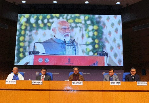
Union Minister for Education, Shri Dharmendra Pradhan, launched the registration portal for the 3rd edition of Kashi Tamil Sangamam (KTS). The Minister, while addressing a press conference, announced that KTS 3.0 will commence on 15th February 2025 in Varanasi, Uttar Pradesh. This 10-day-long event will conclude on 24th February 2025, he added. The portal, kashitamil.iitm.ac.in – hosted by IIT Madras, will accept registrations till 1st February 2025, he added.
Secretary, Ministry of Education, Shri Sanjay Kumar; Principal DG, PIB, Shri Dhirendra Ojha; Additional Secretary, Higher Education, Ministry of Education, Shri Sunil Kumar Barnwal; Chairman, Bhartiya Bhasha Samiti, Shri Chamu Krishna Shastry, and other officials also attended the Press Conference.
Shri Pradhan, while interacting with the media, said that the inseparable bonds between Tamil Nadu and Kashi are set to come alive through Kashi Tamil Sangamam 3.0.
The Minister highlighted that Kashi Tamil Sangamam, a brainchild of Prime Minister, Shri Narendra Modi, is an inspirational initiative to celebrate the timeless bonds between Tamil Nadu and Kashi, strengthen the civilisational links and further the spirit of Ek Bharat Shrestha Bharat.
Shri Pradhan said that Kashi Tamil Sangamam will be a celebration of one of India’s most revered sages—Maharishi Agasthyar. Maharishi Agasthyar’s legacy is deeply woven into India’s cultural and spiritual fabric, Shri Pradhan highlighted. His intellectual brilliance is the bedrock of Tamil language and literature as well as our shared values, knowledge traditions and heritage, he added.
Shri Pradhan said, that this year, Kashi Tamil Sangamam holds a special significance as it is coinciding with the Mahakumbh, and it is also the 1st Sangamam after the ‘Pran Pratishtha’ of Shri Ram Lalla in Ayodhya.
With Maharishi Agasthyar as the central theme and Mahakumbh and Shri Ayodhya Dham as the backdrop, Kashi Tamil Sangamam 3.0 will offer a divine experience and bring Tamil Nadu and Kashi—the two timeless centres of our civilisation and culture, more closer than ever, he said.
Shri Pradhan encouraged people of Tamil Nadu to participate in Kashi Tamil Sangamam 3.0 wholeheartedly.
An exhibition on the different facets of Sage Agasthyar and his contributions to world of Health, Philosophy, Science, Linguistics, Literature, Polity, Culture, Art, particularly to Tamil and Tamil Nadu, etc. and Seminars, workshops, book release, etc. will be organised at Kashi during KTS 3.0. Competitions and other awareness programs in Tamil Nadu prior to KTS 3.0 will be organised in a befitting manner in major cities of India and abroad where there is considerable Tamil diaspora.
This year, the government has decided to bring around 1000 delegates from Tamil Nadu under five categories/groups: (i) Students, Teachers, and Writers; (ii) Farmers and Artisans (Vishwakarma Categories); (iii) Professionals and Small Entrepreneurs; (iv) Women (SHG, Mudra Loan beneficiaries, DBHPS Pracharaks); and (v) Start-up, Innovation, Edu-Tech, Research. This year, an additional group of around 200 students of Tamil origin studying in various CUs will be a part of this event to enliven the bond between Kashi and Tamil Nadu. Participation of youth in all categories will be encouraged this year.
The duration of the tour will be 8 Days (4 for travel, 4 at site). The first group will leave Tamil Nadu on 13th February 2025 and the last group will return to Tamil Nadu on 26th February 2025.
The objective of the Kashi Tamil Sangamam is to rediscover, reaffirm, and celebrate the age-old links between Tamil Nadu and Kashi—two of the country’s most important and ancient seats of learning.
Kashi Tamil Sangamam is being organized by the Ministry of Education, Govt. of India in collaboration with other ministries including Culture, Textiles, Railways, Tourism, Food Processing, I&B etc. and the Govt. of UP. The programme aims to provide an opportunity for scholars, students, philosophers, traders, artisans, artists and people from other walks of life from the two regions to come together, share their knowledge, culture and best practices and learn from each other’s experience. It also aims to make the youth aware and experience cultural oneness. The endeavour is in sync with NEP 2020’s emphasis on integrating the wealth of Indian Knowledge Systems with modern systems of knowledge. IIT Madras and BHU are the two implementing agencies for the programme.
The Government has so far celebrated the Kashi Tamil Sangamam on two occasions earlier; i.e., for one month in 2022 and for a fortnight in 2023 and around 4000 delegates from Tamil Nadu have been a part of this event. In both the editions of KTS, there were overwhelming responses from people of Tamil Nadu and Uttar Pradesh. IIT Madras will be the sender institution and BHU the receiving institution, as in the earlier editions. IIT Madras will call for applications for participation through a portal, which was launched today.
KTS 2.0 was inaugurated by Prime Minister Shri Narendra Modi at Varanasi on 17th December, 2023, with the first-ever real-time, app-based translation of a part of the Prime Minister’s speech in Tamil for the benefit of visiting Tamil delegates.


You must be logged in to post a comment.